Econometrics · Lab 16 of 20
What Happens Around an Eligibility Cutoff?
Regression discontinuity, bandwidths, continuity and local effects.
An academic grant is awarded when a student's eligibility score reaches 50. Students scoring 49.9 and 50.1 receive different treatment even though their scores are almost identical. Could that policy rule help us estimate the grant's effect on first-year credits completed?
This question is narrower than asking whether grant recipients outperform everyone else. Students far above the cutoff may differ substantially from students far below it. Regression discontinuity, or RD, focuses on the change at the threshold while allowing outcomes to vary smoothly with the score on either side. The policy rule supplies the comparison; the regression helps estimate the limits of those smooth relationships.
The dataset is original and entirely synthetic. Its 600 independent observations do not describe actual students, a real grant, or a university. The observations are supplied in scholarship_cutoff.xlsx. The estimates below come from executing lab.py with OpenEconometrics. They illustrate how a design works and how its uncertainty is reported.
1. Distinguish a local comparison from a group comparison
Let be a student's eligibility score and let the cutoff be . Treatment is assigned by the sharp rule
“Sharp” means that the rule determines treatment perfectly in this example: every student at or above the threshold receives the grant, and every student below it does not. An application with imperfect take-up would be a fuzzy RD, with a different estimand and a first-stage discontinuity in actual receipt. We do not silently interpret this sharp example as such a design.
The outcome is credits completed in the first year. Scores and credits have different units: a one-point increase in the eligibility score is not a one-credit increase in academic progress. The RD estimand is
The first term approaches the threshold from the treated side; the second approaches from the untreated side. We are estimating a jump at score 50, not an average difference across the entire score distribution. If the effect varies with academic preparation, this local effect need not equal the effect for students with scores of 25 or 75.
Imagine that outcomes increase with preparation even without a grant. A raw recipient-versus-nonrecipient mean comparison combines that smooth preparation gradient with the policy effect. Comparing fitted limits at the same score removes this particular difference if the underlying untreated relationship continues smoothly through the cutoff.
2. Read the data-generating process as a research design
The supplied synthetic scores were drawn independently over 20–80. Define . The synthetic outcome is generated as
The untreated response is curved but continuous at the threshold. Treatment adds exactly three credits everywhere in this particular simulation, so the true jump at the cutoff is 3.000 credits. The analyst's estimator does not receive that value as an input.
| Variable | Meaning | Unit / coding |
|---|---|---|
student | Independent observation identifier | 0–599 |
score | Running variable determining assignment | Eligibility points, 20–80 |
awarded | Actual grant receipt | 1 if score is at least 50 |
credits | First-year academic progress | Credits completed |
No records are missing, and no sampling weights are applied. The grant is the only discontinuous component in the generator. There is no manipulation of scores and no other policy beginning at score 50. Those are facts about this synthetic construction, not conclusions that a fitted RD model could establish about an empirical program.
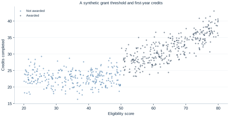
Use the figure to distinguish the continuous slope from the discontinuity. The cloud contains individual noise, so the distance between the two nearest observations is not itself the estimated policy effect. A regression uses several nearby observations to estimate the conditional mean on each side. Likewise, a jump that looks plausible in a graph does not demonstrate that potential outcomes would have been continuous without treatment.
3. Run the complete example, then examine its pieces
Download scholarship_cutoff.xlsx and lab.py. In OpenEconometrics, import the workbook without changing its filename, then open lab.py in a Python document and run the complete file. The workbook's first sheet, Data, contains the observations; Dictionary explains the variables and units.
The script reads the prepared student observations and shows the scatterplot, the native RD result, and a bandwidth comparison table. Everyone using the supplied workbook starts from the same observations and obtains the same reported results.
In ordinary Python, keep the workbook beside lab.py and run python lab.py from an environment where OpenEconometrics is installed. To read a workbook from another folder, use from lab import run_lab, then call run_lab(data_path="/path/to/scholarship_cutoff.xlsx"). The script writes no exports unless an output directory is explicitly supplied.
After the complete script has defined its functions, reload the supplied observations and verify assignment:
data = load_data()
print(data.groupby("awarded").size())
print((data.awarded == (data.score >= 50).astype(int)).all())
There are 280 observations below and 320 at or above the cutoff. These are full-sample counts, not the number effectively used by the local fit. Keeping that distinction prevents a common reporting error: presenting all 600 students as though they all had positive weight in the point estimator.
The main model is explicit about its choices:
rd = oe.rdrobust(
    data=data,
    y="credits",
    running="score",
    cutoff=50.0,
    h=12.0,
    b=18.0,
    p=1,
    q=2,
    kernel="triangular",
    vce="hc0",
    missing="raise",
    alpha=0.05,
)
print(rd.summary())
The point-estimation bandwidth is 12 score points on each side: scores within 38–62 receive positive triangular weight, apart from zero weight at an exact boundary. Here that includes 122 left-side and 127 right-side observations. The separate bias bandwidth is 18 points, which uses a wider neighborhood for estimating curvature. These bandwidths are declared before examining the outcomes; this is not a claim that 12 and 18 are universally optimal choices.
4. Understand local fitting and bias correction
The conventional estimator fits a separate local line on each side. With , the weighted least-squares problem on a side is
Observations closer to the threshold receive more weight. The fitted intercept estimates the side's limit at ; the difference between the two intercepts estimates the jump. Separate slopes allow the relationship between score and credits to differ across the cutoff.
A local line is an approximation to a potentially curved conditional mean. Using more distant observations can reduce variance while increasing approximation bias. In the generator, the quadratic term makes that issue visible. The bias-correction stage fits a quadratic, q=2, using bandwidth b=18, estimates the leading bias of the local linear fit, and subtracts it.
Bias correction is itself estimated from noisy outcomes. Its uncertainty must be included when constructing the robust bias-corrected interval. Treating the corrected point estimate as though the bias adjustment were known can produce an interval that is too optimistic. This distinction motivates the three rows returned by OpenEconometrics:
| Row | Estimate, credits | Standard error | 95% interval |
|---|---|---|---|
| Conventional | 4.198 | 0.734 | [2.760, 5.637] |
| Bias-corrected | 4.579 | 0.734 | [3.141, 6.017] |
| Robust | 4.579 | 0.894 | [2.826, 6.331] |
The last row combines the corrected point estimate with uncertainty that accounts for estimating the correction. It is the main reported interval in this lab. The middle row retains the conventional standard error, so it should not be substituted for the robust interval merely because it is shorter. These are alternative estimates or inference calculations for one local discontinuity, not three distinct treatment effects.
The Robust row uses normal reference inference. Its two-sided p-value is approximately 0.000000304. The estimate is about 4.58 credits at the cutoff, with a robust bias-corrected interval from 2.83 to 6.33. The true simulated three-credit effect lies inside this particular interval. Correction does not guarantee that the corrected point estimate is closer to the truth in each finite sample; here it moves farther from three than the conventional estimate.
5. Investigate bandwidth sensitivity without choosing a favorite answer
The complete script estimates three declared specifications on the same input data. It changes the neighborhood rather than searching for a preferred p-value:
| Main bandwidth | Bias bandwidth | Local point-fit observations | Robust estimate | Robust 95% interval |
|---|---|---|---|---|
| 8 | 12 | 159 | 5.394 | [3.224, 7.564] |
| 12 | 18 | 249 | 4.579 | [2.826, 6.331] |
| 16 | 24 | 334 | 4.234 | [2.710, 5.757] |
A smaller neighborhood uses fewer observations and a more local approximation. A wider one uses more information but relies on smooth approximation over a larger score range. In this sample, the narrow estimate is less precise, and its interval misses the known true value. That is possible even for a sensible inferential procedure. Coverage describes repeated samples, not a guarantee about every displayed interval.
Do not interpret the table as a competition whose winner is the smallest standard error, the largest effect, or the interval that happens to contain three. In an empirical setting the true value is not available. A defensible analysis states how bandwidths were chosen, shows reasonable sensitivity, and reports when conclusions depend strongly on those choices.
6. Separate statistical calculation from causal identification
For a causal interpretation, untreated potential outcomes must be continuous at the threshold, along with the relevant treatment comparison. Students must not be able to sort precisely around the cutoff in a way that changes those potential outcomes discontinuously. Other policies must not change at the same score. There must also be adequate observations and distinct score values on both sides to estimate local limits.
These conditions suggest substantive checks: understand how the score was recorded, inspect unusual bunching or heaping, examine predetermined characteristics around the threshold, and document other eligibility rules. A smooth observed covariate or an unremarkable density plot is informative but does not prove all unobserved determinants are continuous. A large estimated jump cannot compensate for a broken assignment story.
The synthetic design assumes independent students. If real outcomes shared school-level shocks or assignment operated at a school level, uncertainty would need to reflect that dependence rather than copying this HC0 choice. The local estimate also does not tell us the grant's cost effectiveness, its effect on students far from the cutoff, or whether benefits persist beyond the first year. Those are additional questions requiring additional data or designs.
Robust bias-corrected inference addresses local approximation bias and the uncertainty of estimating that bias. It does not correct score manipulation, simultaneous policies, selective outcome observation, or a discontinuous change in the type of student at the threshold. See the original methodological paper by Calonico, Cattaneo, and Titiunik for the inferential distinction developed here.
7. Communicate the local result
The publication LaTeX table keeps the conventional and robust rows together so their different roles remain visible. A report should identify the robust row as its primary inference rather than treating every row as a separate finding.
A useful written interpretation includes the eligibility threshold, the outcome unit, the local population, the bandwidths, and the reported interval. Keep the causal qualification close to the coefficient. “The model reports a 4.58-credit local discontinuity at score 50” is a description of the estimate; attributing that discontinuity to the grant additionally relies on the continuity and assignment arguments above.
Also state whose outcome is being compared. The local comparison concerns students close to the eligibility threshold under the assignment mechanism observed in the data. Extending eligibility to much lower scores would change the population receiving treatment and might also change program capacity, peer effects, or take-up. A precise local discontinuity therefore informs a specific policy margin without answering every expansion question.
8. Questions for your analysis
- Explain why a comparison of all awarded and non-awarded students answers a different question from the RD limit comparison. Use the generator's smooth score terms to make the distinction concrete.
- Derive the conventional estimator as the difference between two local intercepts. Explain why separate slopes are allowed.
- State which observations have positive point-fit weight under
h=12and distinguish their count from the full sample and the bias-fit sample. - Explain why the bias-corrected and robust rows have the same point estimate but different standard errors. Which interval would you report, and why?
- Interpret the three bandwidth specifications without choosing a model by its significance. What uncertainty is suggested by their differences?
- Suppose score 50 also triggers priority course registration. Can this RD separate the grant from that change? State the additional evidence needed.
- Write a short result paragraph that reports the numerical estimate while making its local scope and identifying assumptions explicit.