Causal Effects in Nonexperimental Studies

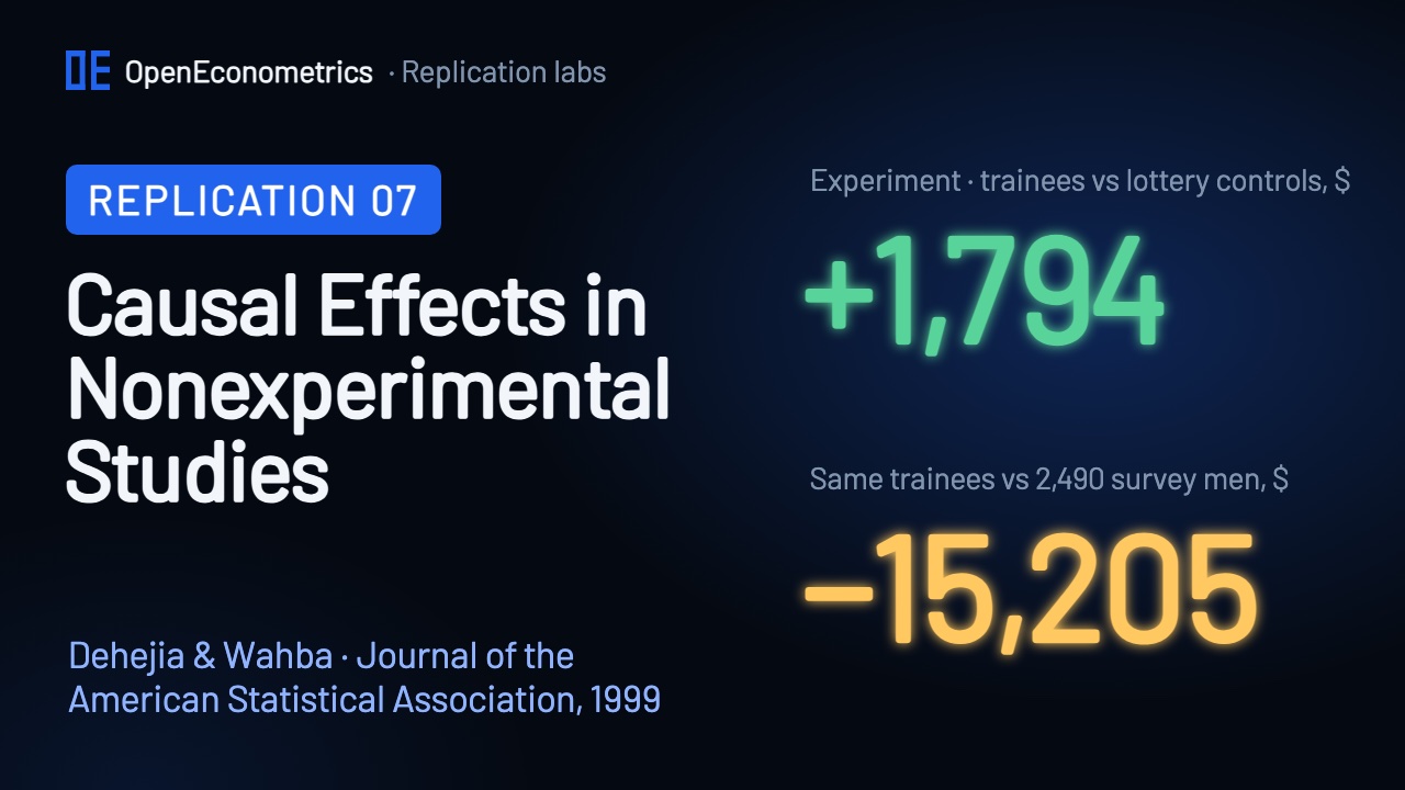
In the mid-1970s the National Supported Work Demonstration assigned job training by lottery, and in 1978 the trainees earned $1,794 more than the randomized controls. Compare the same 185 trainees with 2,490 men from a national survey instead, and the program appears to cut earnings by $15,205. Dehejia and Wahba asked whether propensity-score methods can close that gap without the lottery. This lab rebuilds the paper's five tables and the counts behind its two figures from the authors' posted data in OpenEconometrics, and compares 775 printed numbers with the run. The experimental benchmark, the naive comparisons and the regressions are reproduced exactly. The paper's tight propensity-score range is not, and the reasons are the lesson of this lab: matching is fragile when overlap is thin.

The experiment and the question

The National Supported Work (NSW) Demonstration gave 6 to 18 months of subsidized work to people with weak labor-market records, and a lottery decided which applicants got the program. The paper uses the men for whom earnings in 1974 are also known: 185 trainees and 260 controls. The outcome is earnings in 1978, in 1982 dollars. Because of the lottery, a difference in means is an unbiased estimate of the effect on the trainees.

Experimental estimate, 1978 earnings	Paper	This lab
RE74 subsample · difference in means (185 vs 260)	1,794 (633)	1,794.34 (632.85)
RE74 subsample · with covariates	1,672 (638)	1,672.20 (638.40)
LaLonde's sample · difference in means (297 vs 425)	886 (472)	886.30 (472.09)

The benchmark is $1,794 with a standard error of 633; with covariates it is $1,672 (638), because the lottery balanced them. In LaLonde's larger sample of 297 trainees and 425 controls the effect is $886 (472); the paper attributes the gap to the different make-up of the two samples.

LaLonde (1986) then set the experimental controls aside and asked whether standard econometric methods, applied to men from national surveys, recover the experimental answer. The paper uses his comparison groups: PSID-1, 2,490 men from the Panel Study of Income Dynamics; CPS-1, 15,992 men from the Current Population Survey; and four smaller subsets (PSID-2 and 3, CPS-2 and 3) that LaLonde selected to resemble the trainees more closely.

Mean	Trainees (185)	Controls (260)	PSID-1 (2,490)	CPS-1 (15,992)
Age (years)	25.8	25.1	34.9	33.2
Education (years)	10.3	10.1	12.1	12.0
Black	0.84	0.83	0.25	0.07
Married	0.19	0.15	0.87	0.71
No high-school degree	0.71	0.83	0.31	0.30
Earnings 1974 ($)	2,096	2,107	19,429	14,017
Earnings 1975 ($)	1,532	1,267	19,063	13,651

The two populations hardly overlap. The trainees were about 26 years old, with 10.3 years of schooling; 19% were married and 84% were black, and they earned $2,096 in 1974. The PSID men were about 35, with 12.1 years of schooling; 87% were married, 25% were black, and they earned $19,429. The CPS men were about 33, 71% married, 7% black, with $14,017. Before the program, the survey men earned 7 to 12 times as much as the trainees.

Comparison group	Men	Naive · paper	Naive · lab	Regression · paper	Regression · lab
PSID-1	2,490	−15,205	−15,205	731	731
PSID-2	253	−3,647	−3,647	683	683
PSID-3	128	1,069	1,070	825	825
CPS-1	15,992	−8,498	−8,498	972	972
CPS-2	2,369	−3,822	−3,822	790	790
CPS-3	429	−635	−635	1,326	1,326

The naive comparison is −$15,205 against PSID-1 and −$8,498 against CPS-1, as printed. A regression on age, age squared, schooling, a high-school degree, race and earnings in 1974 and 1975 moves the PSID-1 estimate to $218 and the CPS-1 estimate to $739. Table 3 prints $731 and $972. The lab reproduces both exactly once the square of 1975 earnings is added, a term the table's note does not list. One squared term moves the PSID-1 estimate by $513: with so little overlap, a regression extrapolates, and its functional form decides the answer.

The propensity score

The paper assumes selection on observables: once a man's age, schooling, race, marital status, degree and earnings history are known, whether he trained is as good as random. Rosenbaum and Rubin (1983) showed that it is then enough to compare units with the same probability of treatment given those characteristics, the propensity score. Eight dimensions collapse into one number between 0 and 1.

The score is a logit of the treatment indicator, fitted with oe.logit on the trainees stacked with one comparison group. For PSID-1 the notes to Table 3 list 13 terms, among them squares of age, schooling and earnings and an interaction of race with zero earnings in 1974; PSID-1, the smaller PSID groups and the CPS groups each have their own specification. The paper prints the terms of each logit but not its coefficients.

Before estimating anything, the paper looks at overlap. Comparison men whose score lies below the lowest trainee score are dropped; the rest are compared with the trainees in 0.05-wide bins (Figures 1 and 2).

Trainees (185)PSID-1 men kept (1,146)

For PSID-1 the lab's score drops 1,344 of the 2,490 men (the paper reports 1,333). Of the 1,146 that remain, 915 sit in the lowest bin (paper: 928). Above a score of 0.8 there are 98 trainees, 53% of them, and only 7 PSID men.

Trainees (185)CPS-1 men kept (3,856)

For CPS-1 the score drops 12,136 of the 15,992 men (paper: 12,611); 3,454 of the 3,856 that remain sit in the lowest bin, and above 0.8 there are 36 trainees and 8 CPS men (paper: 35 and 7). Most of each comparison group is irrelevant, and the comparison rests on a few dozen men with high scores.

The paper then uses the score in two ways, both estimating the effect on the trainees. Stratification cuts the score into blocks, compares mean earnings within each block and weights the blocks by their number of trainees. Matching gives each trainee the comparison man with the nearest score, with replacement. Matching balances what it can observe: the matched PSID men earned $1,873 in 1974, against $2,096 for the trainees and $19,429 for all PSID men.

The main results

Experiment · benchmark1,794 (633)

PSID-1 · stratification2,156 (1,865)

PSID-1 · matching552 (954)

PSID-2 · stratification1,374 (1,861)

PSID-2 · matching871 (887)

PSID-3 · stratification−98 (1,778)

PSID-3 · matching1,534 (962)

CPS-1 · stratification1,485 (955)

CPS-1 · matching730 (800)

CPS-2 · stratification1,659 (1,450)

CPS-2 · matching1,399 (852)

CPS-3 · stratification1,512 (1,730)

CPS-3 · matching−544 (907)

Lab estimates with 95% intervals. Grey: experiment. Blue: stratification. Amber: matching.

Comparison group	Strata · paper	Strata · lab	Match · paper	Match · lab	Support · paper	Support · lab
PSID-1	1,608 (1,571)	2,156 (1,865)	1,691 (2,209)	552 (954)	1,255	1,331
PSID-2	2,220 (1,768)	1,374 (1,861)	1,455 (2,303)	871 (887)	389	302
PSID-3	2,321 (1,994)	−98 (1,778)	2,120 (2,335)	1,534 (962)	247	245
CPS-1	1,713 (1,115)	1,485 (955)	1,582 (1,069)	730 (800)	4,117	4,041
CPS-2	1,543 (1,461)	1,659 (1,450)	1,788 (1,205)	1,399 (852)	1,493	1,372
CPS-3	1,252 (1,617)	1,512 (1,730)	587 (1,496)	−544 (907)	514	506

The direction of the paper's result holds everywhere. Once the comparison groups are trimmed to the overlap, every estimate moves from large negative numbers to the neighbourhood of the benchmark. The precision does not. For PSID-1 the paper prints $1,608 for stratification and $1,691 for matching; the lab gets $2,156 (1,865) and $552 (954). For CPS-1 the paper prints $1,713 and $1,582; the lab gets $1,485 (955) and $730 (800). Across the six groups the lab's estimates run from −$544 to $2,156, the paper's from $587 to $2,321, and every one of these estimates, the lab's and the paper's, has a standard error of $800 or more.

On its final page, the paper summarizes the PSID-1 and CPS-1 estimates as ranging from $1,473 to $1,774. The lab's eight corresponding estimates, stratification and matching with and without covariates, range from $495 to $2,156.

Why the score-based estimates move

Three details that drive these columns are not published. The logit coefficients: the lab fits the printed specifications, and its scores are close to the authors' but not equal, as the counts above show. The strata: the lab starts from five blocks of width 0.2 and splits a block while the mean score of trainees and comparison men differs at the 1% level, which gives 7 strata for PSID-1 and 8 for CPS-1. The tie rule: when two comparison men are equally close to a trainee, the paper does not say which it uses; the lab lets them share the match. None of these choices was tuned to the printed numbers.

Single-neighbour matching amplifies small differences in the score. The lab's 185 trainees are matched to only 57 different PSID-1 men (the paper's matched sample has 56) and 155 CPS-1 men (paper: 119). Above 0.8, 7 PSID men face 98 trainees, so each is used again and again, and a slightly different score makes a different man the nearest.

PSID-1 · 1 neighbour552 (1,277)

PSID-1 · 2 neighbours1,540 (1,017)

PSID-1 · 5 neighbours2,133 (824)

CPS-1 · 1 neighbour648 (876)

CPS-1 · 2 neighbours902 (756)

CPS-1 · 5 neighbours1,724 (674)

oe.teffects(method="psmatch") with Abadie–Imbens standard errors. The CPS-1 values use the SDK's handling of tied scores.

With one neighbour the PSID-1 estimate is $552 (Abadie–Imbens standard error 1,277); with two, $1,540 (1,017); with five, $2,133 (824). More neighbours shrink the interval but bring in worse matches. For CPS-1 the same three estimates are $648, $902 and $1,724.

The CPS-1 values in that chart expose a tie problem in the SDK itself. CPS-1 contains many men with identical covariates, and so identical scores in principle, but oe.teffects computes their scores with differences in the last digits, so its documented rule that equally distant units share a match is not applied to them. Its single-neighbour estimate, $648, is $83 below the $730 of the matched sets the lab builds itself. The lab reports the matched-set estimate and keeps the SDK value in results.json; in every PSID sample, and in CPS-2 and CPS-3, the two agree.

Score specification (Table 5)	Strata · paper	Strata · lab	Match · paper	Match · lab
PSID-1 · Table 3 score	1,608	2,156	1,691	552
PSID-1 · without squares	1,524	2,277	2,281	1,422
PSID-1 · also without the interaction	1,237	1,342	1,140	2,126
PSID-1 · without 1974 earnings	−869	−848	1,727	1,710
CPS-1 · Table 3 score	1,713	1,485	1,582	730
CPS-1 · without higher powers	1,452	1,454	835	1,036
CPS-1 · also without interactions and zero-earnings dummies	1,299	1,362	1,103	1,794
CPS-1 · without 1974 earnings	1,234	1,411	1,402	1,203

The paper's own sensitivity checks in Table 5 move as well. Simpler PSID-1 scores move its matching estimate from $1,691 to $2,281 and $1,140; the lab's run gives $552, $1,422 and $2,126. Both swing by more than a thousand dollars. Without 1974 earnings, the PSID-1 stratification estimate turns negative in both: −$869 in the paper and −$848 in the run. One year of earnings history is not enough for PSID-1.

Jeffrey Smith and Petra Todd revisited these data in "Does matching overcome LaLonde's critique of nonexperimental estimators?" (Journal of Econometrics 125(1–2), 305–353, 2005, doi:10.1016/j.jeconom.2004.04.011) and found the matching estimates sensitive to the choice of sample and specification.

Effect on the trainees (extension)	PSID-1	CPS-1
Experimental benchmark	1,794 (633)	1,794 (633)
Matching, one neighbour (lab)	552 (954)	730 (800)
Inverse-probability weighting	3,028 (880)	1,782 (779)
Augmented IPW	3,775 (1,309)	1,659 (805)

Weighting instead of matching shows the same overlap problem from another side. Inverse-probability weighting gives $1,782 (779) for CPS-1, near the benchmark, but $3,028 (880) for PSID-1, more than one standard error above it, because the few PSID men with high scores receive enormous weights. Augmented IPW gives $1,659 (805) and $3,775 (1,309).

The scorecard

Target	Paper	This lab	Result
Table 3 · experiment · difference in means	1,794 (633)	1,794.34 (632.85)	✓ Match
Table 3 · experiment · with covariates	1,672 (638)	1,672.20 (638.40)	✓ Match
Table 3 · PSID-1 · difference in means	−15,205 (1,154)	−15,204.78 (1,154.61)	✓ Match
Table 3 · CPS-1 · difference in means	−8,498 (712)	−8,497.52 (712.02)	✓ Match
Table 3 · PSID-1 · regression (with RE75²)	731 (886)	731.36 (885.91)	✓ Match
Table 3 · CPS-1 · regression (with RE75²)	972 (550)	972.08 (549.57)	✓ Match
Table 3 · PSID-1 · stratification	1,608 (1,571)	2,156.02 (1,864.55)	Difference
Table 3 · PSID-1 · matching	1,691 (2,209)	552.29 (954.28)	Difference
Table 3 · CPS-1 · stratification	1,713 (1,115)	1,485.28 (954.53)	Difference
Table 3 · CPS-1 · matching	1,582 (1,069)	730.38 (800.24)	Difference
Figure 1 · PSID-1 men below the lowest trainee score	1,333	1,344	Difference
All tables and figure counts	775 numbers	354 match · 36 rounding · 385 differ	Difference

Table	Numbers	Match	Rounding	Differ
Table 1 · Sample means	166	132	19	15
Table 2 · LaLonde's regressions	210	170	1	39
Table 3 · Main results	94	12	5	77
Table 4 · Matched samples	111	10	1	100
Table 5 · Sensitivity	184	29	10	145
Figure 1 · PSID-1 counts	5	1	0	4
Figure 2 · CPS-1 counts	5	0	0	5
All	775	354	36	385

Of the 775 printed numbers, 354 match at the printed precision and 36 differ only in the last digit, mostly because the paper truncates instead of rounding. 385 differ, and each one is kept with a diagnosis. The split that matters is by whether a number depends on the estimated score:

• 465 numbers do not depend on the score. 349 match, 36 round, and of the 80 that differ, 76 are reproduced by a documented alternative.
• 310 numbers depend on the score. 5 match and 305 differ.

The 385 differences fall into five classes:

• 12 covariance. Every standard error in parentheses in Table 1 divides the group's standard deviation by √425, the size of LaLonde's control group, rather than by the group's own size.
• 1 published typo. Table 1 prints the PSID-3 Hispanic share as .18; the data give .12, as Dehejia's data page itself says.
• 12 published inconsistencies. Table 3's regression column prints the regression of Table 2's column 5, not the one its note describes, and one Table 2 cell differs from the same regression in Table 5.
• 124 specification. The unpublished strata (71), and two regression columns that need a term the notes do not list (38 and 15).
• 236 unexplained. 2 are in Table 1; all others depend on the estimated score. They are close to the paper but never equal.

Where this replication stops

The paper's 1999 estimation code is not available, and it prints neither the logit coefficients nor the strata nor the tie rule, so every score-based number here comes from documented choices made by the lab, never tuned to the printed values. The figures' bar heights are not labelled in the paper; only the counts stated in the captions and text are compared, and the overlap charts above draw the lab's own bins. The selection-on-observables assumption cannot be tested with these data beyond the paper's own sensitivity checks. Dehejia and Wahba (2002, Review of Economics and Statistics 84, 151–161) is a different paper with different tables and is not compared. The weighting estimates are extensions, not paper targets.

Run it yourself

Watch the companion video above. The lab package will be published here. Rajeev Dehejia's data page distributes the files for attributable non-commercial use under Creative Commons Attribution-NonCommercial 2.0 (CC BY-NC 2.0) and asks users to cite Dehejia and Wahba (1999), Dehejia and Wahba (2002) and LaLonde (1986). The lab downloads them and never redistributes them:

1. Run prepare_sources.py from the lab package. It downloads the 8 Stata files (the NSW samples and the six comparison groups) from the data page and checks each one against its recorded SHA-256 fingerprint.
2. Open a Python document in OpenEconometrics, point the launcher at the lab, the downloaded files and a new results folder, and press Run.

from lab import run_lab

result = run_lab(
    source_root=source_dir,
    output_dir=results_dir,
    display_callback=display,
)

The run fits 18 propensity-score models with their strata and matches. Matching on the score is one call:

oe.teffects(data=psid, y="re78", treatment="treat", tx=LOGIT["e"], method="psmatch", estimand="atet", neighbors=1, pstolerance=1e-300)

The run writes reconciliation.csv, with every printed number next to the lab's result and a diagnosis for each difference.

The paper

Rajeev H. Dehejia and Sadek Wahba, "Causal Effects in Nonexperimental Studies: Reevaluating the Evaluation of Training Programs", Journal of the American Statistical Association 94(448), 1053–1062, 1999. doi:10.1080/01621459.1999.10473858. It revisits Robert J. LaLonde, "Evaluating the Econometric Evaluations of Training Programs with Experimental Data", American Economic Review 76(4), 604–620, 1986. The paper and the authors' data keep their own rights; this page and the lab describe and recompute them.