A Theory of Falling Growth and Rising Rents

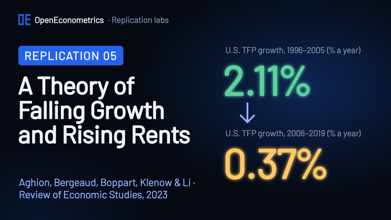
Productivity in U.S. manufacturing, trade and services grew by 0.79% a year in 1988–1995, by 2.11% in 1996–2005 and by only 0.37% in 2006–2019. Over the same years the largest firms took a bigger share of sales. Aghion, Bergeaud, Boppart, Klenow and Li explain both with one shock: running many product lines became cheaper for the most efficient firms. Like Replication 01, The Simple Macroeconomics of AI, this is a quantitative-theory paper. This lab recomputes its data facts with OpenEconometrics estimators, runs the authors' own Python code for the calibrated model, and checks all 114 printed numbers in Tables 2–13 against the paper and against the authors' output workbook.

A burst, then a slowdown

Figure 1 of the paper is total factor productivity (TFP) growth in Manufacturing, Trade and Services from the BLS industry accounts in the authors' package, with R&D and other intangible investment added back and divided by labour's share of costs (labour-augmenting form). The lab rebuilds the 32 annual values, 1988 to 2019; 1987 is the base year of the first log difference.

Annual growthPeriod mean

The period means are 0.79% a year over the 8 years 1988–1995, 2.11% over the 10 years 1996–2005 and 0.37% over the 14 years 2006–2019, as printed. oe.tabstat computes them, and a regression on three period dummies without a constant gives the same values.

The paper reports no standard errors. As an extension, the lab estimates that regression with oe.newey (Newey–West, 3 lags) and tests the differences with oe.lincom. The acceleration of 1.31 points (SE 0.26) and the deceleration of 1.74 points (SE 0.23) are far from zero. The long-run change from the first period to the last, −0.42 points (SE 0.21, p = 0.05), is measured much less precisely, and it is the number the model is asked to explain.

Acceleration · 1996–2005 minus 1988–19951.31 (0.26)

Deceleration · 1996–2005 minus 2006–20191.74 (0.23)

Long-run change · 2006–2019 minus 1988–1995−0.42 (0.21)

Extension, not in the paper: oe.newey with 3 lags on three period dummies, then oe.lincom. Values are estimates with Newey–West standard errors; bars are the 95% intervals oe.lincom reports.

Concentration is the sales share of the top 0.374% of firms, the size of the top 20 firms in an average four-digit industry. It rose in all four sectors between 1987 and 2012, from 69.9% to 88.7% in retail and from 36.0% to 38.5% in manufacturing. Weighted by sector, it rose from 45.9% to 58.0%. Over the same years the labour share in these sectors fell by 5.97 percentage points.

Sales share of the top 0.374% of firms	1987	2012	Change (points)
Retail	69.9	88.7	+18.8
Services	50.9	66.3	+15.3
Wholesale	45.4	57.5	+12.2
Manufacturing	36.0	38.5	+2.5
Four sectors, weighted	45.9	58.0	+12.1

A model of creative destruction

The economy is a continuum of product lines, each supplied by the firm with the best quality. An innovator raises quality by a step γ and takes the line over. If a share z of lines changes hands each year, growth is g = z · ln γ: at the calibration, 3.6% of lines a year and γ = 1.246 give the 0.79% of the data.

A few firms, 0.374% of them, are efficient: their costs are lower by a factor Δ = 1.183. A leader prices just below the cost of its runner-up, the firm whose product it replaced, so its markup depends on who that runner-up is.

Leader	Runner-up	Markup	At the calibration
Efficient	Ordinary	γΔ (quality and cost)	1.473
Same type	Same type	γ (quality only)	1.246
Ordinary	Efficient	γ/Δ	1.054

Running many lines is costly: a firm's overhead rises with the square of the number of lines it runs, scaled by ψo, and efficient firms expand until one more line no longer pays for its overhead. A second parameter, ψr, sets the cost of research.

The mechanism follows. If ψo falls, efficient firms innovate to take over more lines, and growth bursts. Once they hold more lines, every innovator is more likely to face an efficient runner-up: markups within firms fall, the reward for innovating falls, and long-run growth ends lower. Because sales shift towards efficient, high-markup firms, concentration and the share of rents in GDP rise.

Calibration

The share of efficient firms is set directly. Five parameters (ψo, Δ, γ, ψr and the discount factor β) are chosen to match five targets in Table 2.

Table 2 target	Data (lab)	Model (lab)	Paper: data / model
Top-20 percentile (%)	0.374	0.374	0.374 / 0.374
Sales share of the top 20 (%)	45.89	45.92	45.9 / 45.9
Labour share vs size	−3.07	−3.07	−3.07 / −3.07
Markup (Hall 2018)	1.2347	1.2373	1.24 / 1.24
Productivity growth (%)	0.793	0.793	0.79 / 0.79
Real interest rate (%)	6.09	6.10	6.10 / 6.10

The model matches every target at the printed precision. The data column comes from the package's data, and all 154 cells of the authors' data-moments sheet are reproduced. Two data targets are carried rounded by the scripts: Hall's (2018) markup is 1.2347, the code uses 1.235 and the paper prints 1.24, while Farhi and Gourio's real rate is 6.0895%, carried as 6.1% and printed as 6.10.

The authors search a grid of 12,800,000 parameter combinations and then run a chain of up to 200 constrained optimisations from the best grid point. The fit is close but not exact: at the saved calibration (Table 3: ψo = 1.1·10⁻³, Δ = 1.183, γ = 1.246, ψr = 1.460, β = 0.950) the weighted distance to the targets is 0.000226. As the authors' README instructs, the lab computes the tables from this saved calibration.

Two balanced growth paths

To match the 12.1-point rise in concentration, ψo must fall by 19.4% (Table 4). That lowers long-run growth, but not by the 0.42 points of the data, so the research cost ψr is also raised by 10.5%. The authors' bisections find both changes, and the lab reruns them from the saved calibration.

Table 8	Initial	Ending · ψo, ψr	Ending · Δ, ψr
Concentration S* (% of lines)	45.92	58.00	58.00
Creative destruction z* (%)	3.61	1.68	1.68
Growth (%)	0.79	0.37	0.37
Aggregate markup μ	1.237	1.237	1.233
Markup, efficient firms μH	1.359	1.332	1.352
Markup, ordinary firms μL	1.150	1.127	1.099
Real interest rate (%)	6.10	5.65	5.65
R&D / GDP (%)	5.27	2.71	2.18
Overhead / GDP (%)	3.11	3.99	4.95
Rents / GDP (%)	10.80	12.48	11.77

Concentration rises from 45.9% to 58.0% of lines, creative destruction falls from 3.6% to 1.7% of lines a year, and growth falls from 0.79% to 0.37%. Markups within firms fall, from 1.36 to 1.33 for efficient firms and from 1.15 to 1.13 for ordinary ones, yet the aggregate markup stays at 1.24 because sales shift to the efficient firms. R&D falls from 5.3% to 2.7% of GDP, overhead rises from 3.1% to 4.0%, and rents (output minus wages, R&D and overhead) rise from 10.8% to 12.5%. The real interest rate falls from 6.1% to 5.7%.

Change in long-run growth (points)	Cheaper overhead ψo (Table 5)	Wider gap Δ (Table 7)
1. Both changes	−0.424	−0.424
2. Only the R&D cost ψr	−0.186	0.247
1 minus 2	−0.238	−0.671
3. Only the driving force	−0.263	−0.595
Contribution (average)	−0.251	−0.633

Together the two changes lower growth by 0.42 points and the higher research cost alone by 0.19. The overhead effect is either the difference (−0.24) or the overhead change on its own (−0.26); the paper averages them to −0.25, more than half of the slowdown.

Labour share, change (points)	Total	Within firms	Between firms
Data, 1987–2012	−5.97	+1.65	−7.62
Model · ψo, ψr	−0.01	+2.19	−2.20
Model · Δ, ψr	+0.34	+4.89	−4.55

In the data the labour share fell by 5.97 points: +1.65 within firms and −7.62 between them. The model has both forces, +2.19 within firms as markups fall and −2.20 between them, but they almost cancel (−0.01).

The transition

The authors' transition_RF.py solves the economy year by year after the shock. The lab records all six paths and the series behind Figures 2 to 5.

Overhead cost ψo falls 19.4% (Figure 2)Efficiency gap Δ widens 4.0% (Figure 4)

When ψo falls, growth jumps from 0.79% to a peak of 2.48% in year 1 and then settles at a new long-run rate of 0.53%; concentration is close to its new level within five years. A wider efficiency gap gives a peak of 2.67% and a new long-run rate of 0.20%.

Old balanced growth pathAfter the overhead decline (Figure 3)

Consumption first drops by 5.6%, as efficient firms spend on research and overhead, is above the old path from year 2 to year 24, and then falls behind for good. Over the whole path the overhead decline is worth a permanent loss of 0.12% of consumption (Table 11).

A wider efficiency gap

The paper also asks whether a wider cost advantage of efficient firms, rather than cheaper overhead, could drive the same facts. To match the rise in concentration, Δ must rise by 4.0% (Table 6). This force is stronger: on its own it lowers long-run growth by 0.60 points, and by 0.63 in the paper's averaged measure (Table 7), more than the data, so the research cost must now fall by 11.2% (alone, that would raise growth by 0.25 points). Markups within ordinary firms fall further, to 1.10, and rents rise to 11.8% of GDP.

Tables 10–13	Data	Cheaper overhead ψo	Wider gap Δ
Acceleration (points)	1.31	0.31 (24.0%)	0.32 (24.4%)
Deceleration (points)	1.74	0.56 (32.4%)	0.95 (54.8%)
Welfare, consumption equivalent (%)	—	−0.12	−3.28

The acceleration is average growth over the ten years after the shock minus growth before it, and the deceleration is that average minus the new long-run growth; in the data they are 1.31 and 1.74 points. Cheaper overhead accounts for 0.31 points of the acceleration (24.0%) and 0.56 points of the deceleration (32.4%). A wider gap explains 24.4% and 54.8%, but at a permanent cost of 3.28% of consumption, against 0.12% for cheaper overhead, and consumption falls back below the old path sooner, after year 18.

The scorecard

Target	Paper	This lab	Result
Figure 1 · TFP growth 1996–2005	2.11%	2.1067%	✓ Match
Table 3 · quality step γ	1.246	1.2459	✓ Match
Table 4 · overhead cost ψo, change	−19.4%	−19.3562%	✓ Match
Table 5 · ψo contribution to growth	−0.25	−0.2508	✓ Match
Table 8 · rents / GDP, ending (ψo)	12.5	12.4843	✓ Match
Table 10 · deceleration explained	(32.4%)	(32.4476%)	✓ Match
Table 11 · welfare, ψo contribution	−0.12%	−0.1175%	✓ Match
Table 2 · markup target (data)	1.24	1.2347	Rounding
Table 12 · deceleration, Δ and ψr	0.94	0.945008	Rounding
Tables 2–13 · every printed number	114	110 match · 4 rounding	Rounding
Authors' workbook · Tables 2–13	114	103 match · 11 differ	Difference
Figure A1b · TFP growth 2006–2019	1.16%	1.2459%	Difference

All 114 printed numbers in Tables 2–13 are reproduced: 110 match at the printed precision and 4 under a named rounding convention, and none differs. Two of the four are the data targets above. The other two are in the joint Δ-and-ψr transition. The authors' workbook keeps every digit, and against it 103 of the 114 numbers match; the 11 that differ are all in Tables 12 and 13.

• Solver drift in one path. Five of the six transition paths agree with the workbook to at least 7 significant digits. In the path in which Δ and ψr change together, each of the 11 cells differs from the workbook by less than 0.0001 in absolute or in relative terms: its acceleration is 0.521053 here and 0.521030 in the workbook. transition_RF.py solves every year with SciPy's L-BFGS-B, the package pins SciPy 1.9.1 and the lab runs 1.18.1. The deceleration of that path is 0.945008 here and 0.944985 in the workbook; the paper prints 0.94, which this run matches only by truncation.
• Table 13, column 3. The paper prints −3.96, which is not the half-up rounding of the authors' own −3.966864 (−3.966793 here); it equals 0.04 − 4.00, the difference of the rounded columns 1 and 2.
• Two calibrations in one package. The workbook's Tables 2–9 come from another calibration (γ = 1.244 and ψr = 1.441, against the printed 1.246 and 1.460). The lab reproduces those sheets from their own parameters and the paper from the saved calibration.
• Figure A1b. For non-farm business TFP growth in 2006–2019 the lab gets 1.25%, as in the package's own figure file; the October 2022 Online Appendix prints 1.16% for a bar labelled 2005–2018. With the package data, 2006–2018 averages 1.20%, so the printed bar comes from an earlier BLS release.
• Footnote 30. The package has no code for it. The printed planner formula gives an optimal growth rate of 9.70% falling to 9.68% after the overhead decline; the footnote prints 9.69%.

Where this replication stops

The tables come from the authors' saved calibration, not from a new one. A rerun of their calibration_RF.py (--calibration-rerun, kept out of the default run) reproduces the 12,800,000-point grid stage to every digit. The second stage does not finish with SciPy 1.18.1: its first run improves the fit to 0.000166, the next 11 leave the region where the model can be solved, and run 13 stops with ValueError: array must not contain infs or NaNs. The calibrated parameters therefore cannot be regenerated here.

The printed targets come from the authors' manuscript of 14 October 2022, which their replication README links as the latest version. The typeset REStud article sits behind a publisher bot check that the lab did not bypass, so the targets were not confirmed against it. Every printed number in Tables 2–9 agrees with the authors' code at the saved calibration.

The lab also takes some inputs as given: the concentration, labour-share and decomposition estimates of Autor and coauthors (2020), Farhi and Gourio's (2018) discount factor and Hall's (2018) Lerner indices, which are checked against his workbook but not re-estimated. Table 1, the online appendix's extensions and the figure PDFs are not rebuilt; the series behind Figures 2 to 5 are exported but have no printed values to compare.

The model itself is a stylised two-type economy. Its driving force is inferred from the rise in concentration, not measured, and it explains about a quarter of the burst and a third to a half of the slowdown.

Run it yourself

Watch the companion video above. The lab package will be published here. The authors' package is on Zenodo under CC BY 4.0:

1. Run prepare_sources.py --destination <new folder> from the lab package. It downloads Replication.zip from the authors' Zenodo record, checks it, and extracts the 32 files the lab needs, each against its recorded SHA-256 fingerprint. Compiled Python files in the archive are never extracted.
2. Open a Python document in OpenEconometrics, point the launcher at the lab, the authors' files and a new results folder, and press Run. The run takes about seven CPU minutes, almost all of it the authors' transition code.

from lab import run_lab

result = run_lab(
    source_root=source_dir,
    output_dir=results_dir,
    display_callback=display,
)

The data facts are a few OpenEconometrics calls, for example oe.newey(data=annual, y="tfp_growth", x=["p0", "p1", "p2"], intercept=False, lag=3, time="year"). The run writes reconciliation.csv, with every printed number, the workbook value and the lab's result side by side.

The paper

Philippe Aghion, Antonin Bergeaud, Timo Boppart, Peter J. Klenow and Huiyu Li, "A Theory of Falling Growth and Rising Rents", Review of Economic Studies 90(6), 2675–2702, 2023. doi:10.1093/restud/rdad016. Replication package: doi:10.5281/zenodo.7459498, CC BY 4.0. Printed values are taken from the authors' manuscript of 14 October 2022 and its Online Appendix.