The Incumbency Advantage in U.S. House Elections

The party that holds a seat in the U.S. House of Representatives usually keeps it. Is that because holding the seat helps, or because parties hold the seats where their voters already are? David Lee answered with elections decided by a hair: where the Democrats barely won and where they barely lost, who won is close to a coin flip. This lab reruns Tables I and II of the paper from Lee's own Stata program and data files in OpenEconometrics, compares all 245 printed numbers with the run, and explains every difference. The printed numbers come from Lee's final working paper of June 2005; the journal version is paywalled, and its tables may differ.

Does holding a seat help a party win it again?

Incumbent partyWinning candidate, next electionRunner-up, next election

Between 1948 and 1998, the incumbent party won the next election in 90% of districts on average over 21 election years. The rate was lowest in 1948, at 79.5%, and highest in 1988, at 96.9%. All 71 plotted values equal Lee's own series.

The analysis sample has 6,558 House elections from 1948 to 1996, seen from the Democrats' side. Years ending in 0 and 2 are left out because districts are redrawn after each census. The Democrats won 3,818 of these elections and lost 2,740. Where they won, their vote share at the next election averaged 0.698; where they lost, 0.347. A naive comparison would call the gap of 0.351 the advantage of holding the seat. But winners and losers differed before the election too: where the Democrats won, they had averaged 0.681 of the vote in the election before and had won 89% of those races; where they lost, 0.368 and 11%. Parties win where they are already strong.

Close elections as an experiment

Lee's running variable is the margin: the Democratic vote share minus the share of the strongest opponent in election t. Above zero the Democrat wins. Within five points of zero there are 322 narrow Democratic wins and 288 narrow losses. Candidates can campaign, raise money and choose where to run, but no one controls the final count to a fraction of a percent. If each candidate's vote share has some randomness, with a smooth density, then just above and just below zero the winner is as good as randomly assigned.

That has a consequence that can be tested, and it is the paper's main contribution: like a randomized experiment, the design implies that everything fixed before election t is balanced at the threshold. If one party could push itself over the line in close races, the earlier vote share, past wins and the candidates' experience would jump at zero.

The estimate comes from one regression of the outcome on a dummy D for a Democratic win in t, a fourth-order polynomial in the margin and the same polynomial times D. Each side of zero gets its own curve, and the coefficient on D is the jump between them at zero: the effect of barely winning. Districts appear several times per decade, so standard errors are clustered by state × district × decade, with 2,618 clusters.

The main result

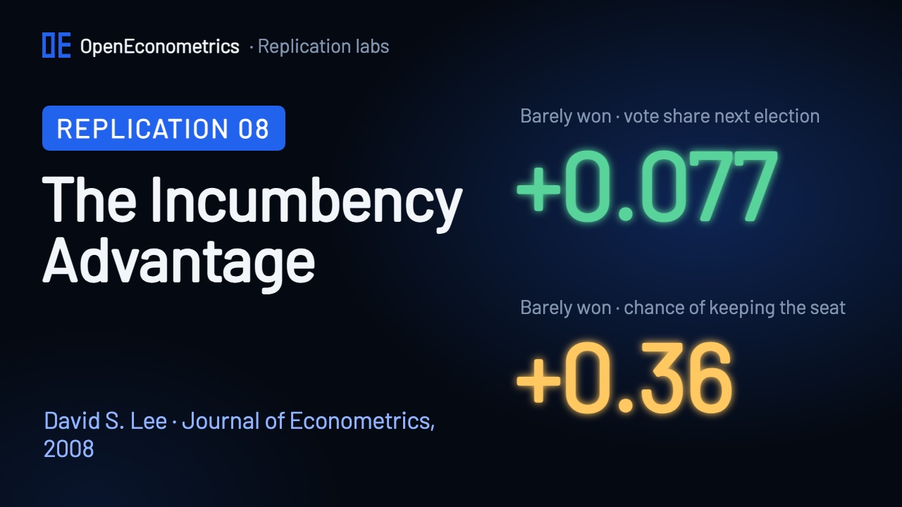
Where the Democrats barely lost, they get 45.4% of the vote at the next election; where they barely won, 53.1%. Table II, column 1, measures the jump: 0.0766, with a clustered standard error of 0.0114, against 0.077 (0.011) printed. Barely winning is worth 7.7 percentage points of vote share at the next election; Lee's text says about 7 or 8 percent. The coefficient equals the difference between Table I's two fits at zero, 0.531 − 0.454, as the paper says it must, and the run checks that identity.

The chance of winning the seat again jumps from 0.247 where the Democrats barely lost to 0.611 where they barely won: a jump of 0.364. The paper prints 0.253 and 0.611, a jump of 0.358, and its text calls the effect about 0.35. This outcome rests on a variable the lab had to rebuild, which explains the loser side. For the 9,674 Democratic candidates themselves (Figure IIa), barely winning raises the chance that the same person runs again and wins from 0.144 to 0.578, a jump of 0.434; Lee calls the effect enormous, about 0.45. That jump includes the decision to run again, which the paper's Figure IIb studies; its variable is not in the posted files.

Balance, placebo and robustness

Table I	All · won	All · lost	±5 points · won	±5 points · lost	At zero · won	At zero · lost
Vote share, t+1	0.698	0.347	0.542	0.446	0.531	0.454
Won, t+1	0.912	0.092	0.683	0.200	0.611	0.247
Vote share, t−1	0.681	0.368	0.501	0.474	0.477	0.481
Won, t−1	0.889	0.109	0.501	0.365	0.419	0.416
Democrat political experience	3.81	0.26	1.66	0.99	1.22	1.18
Opposition political experience	0.24	2.88	1.18	1.34	1.42	1.29
Democrat electoral experience	3.94	0.46	1.95	1.28	1.49	1.47
Opposition electoral experience	0.40	3.01	1.37	1.53	1.62	1.50

Within five points of zero, winners and losers still differ before the election: a previous vote share of 0.501 against 0.474, and Democratic political experience of 1.66 against 0.99. At the threshold itself the gaps disappear: 0.477 against 0.481, and 1.22 against 1.18. Every pre-election variable in Table I is balanced at zero, and every one of their numbers matches the paper. A narrow window is not enough; the trend in the margin has to be accounted for.

Winning in t cannot change the vote share in t−1, so there should be no jump, and there is none: 0.481 on the left and 0.477 on the right. Table II, column 8, turns this into a regression: the coefficient on victory is −0.0018 with a standard error of 0.0107, against −0.002 (0.011) printed, an "effect" of −0.2 points on the past. Winning in t−1 is balanced too (0.419 against 0.416), and the paper's column 8 check for it, −0.005 (0.033), reproduces as −0.0046 (0.0328).

(1) Quartic in the margin only0.0766 (0.0114)

(2) + vote share and win, t−10.0777 (0.0108)

(3) + political experience0.0765 (0.0114)

(4) + electoral experience0.0765 (0.0114)

(5) + all six covariates0.0775 (0.0109)

(6) Residualized vote share, t+10.0808 (0.0136)

(7) Change in vote share, t−1 to t+10.0788 (0.0134)

(8) Placebo: vote share, t−1−0.0018 (0.0107)

Columns 1 to 7: outcomes after election t. Column 8, in amber: the vote share before it, a placebo. Standard errors clustered by state × district × decade.

Adding the pre-election variables leaves the estimate in place, 0.0777 with the previous vote share and win and 0.0775 with all six, and the standard error falls from 0.0114 to 0.0108, as baseline controls should in an experiment. Column 6 runs the discontinuity on what is left of the next vote share after a regression on the six covariates (0.0808), and column 7 uses the change in vote share from t−1 to t+1 (0.0788); Lee writes that the advantage remains at about 8 percent. All 30 coefficients, 30 standard errors and the sample size in Table II match the paper.

Extension, not in the paper	Estimate	95% interval
rdrobust · vote share t+1 · conventional	0.0635 (0.0110)	–
rdrobust · vote share t+1 · robust bias-corrected	0.0591	[0.034, 0.084]
rdrobust · clustered by state × district × decade	0.0591	[0.035, 0.084]
rdrobust · placebo, vote share t−1	−0.0004	[−0.029, 0.028]
rdrobust · won t+1 (rebuilt variable)	0.380	[0.282, 0.477]
rdhonest · points of vote share · M = 0.143	5.85	[2.65, 9.05]
rdhonest · points of vote share · M = 0.1	5.94	[2.87, 9.00]
rddensity · density left / right of zero	0.889 / 1.075	p = 0.152

The extensions use estimators that postdate the paper. oe.rdrobust fits a local linear regression on each side with a triangular kernel and a bandwidth chosen by the data, 0.134, with 782 losses and 804 wins inside it: the jump is 0.0635 (0.0110), and the robust bias-corrected 95% interval is [0.034, 0.084], or [0.035, 0.084] with clustering. The placebo gives −0.0004. The Cattaneo–Jansson–Ma density test in oe.rddensity finds no evidence that elections pile up just above zero (densities 0.889 and 1.075, p = 0.152), though no test can rule sorting out. The honest interval of oe.rdhonest is 5.85 points, [2.65, 9.05], for the rule-of-thumb bound M = 0.143. The local estimates, about 6 points, are smaller than the paper's global quartic, 7.7 points; all are far from zero. The SDK has no Imbens–Kalyanaraman bandwidth selector and no McCrary (2008) density test; Lee's paper uses neither.

The scorecard

Target	Paper	This lab	Result
Table II (1) · victory · quartic in the margin only	0.077 (0.011)	0.0766 (0.0114)	✓ Match
Table II (5) · victory · with all six covariates	0.078 (0.011)	0.0775 (0.0109)	✓ Match
Table II (6) · victory · residualized vote share, t+1	0.081 (0.014)	0.0808 (0.0136)	✓ Match
Table II (7) · victory · change in vote share, t−1 to t+1	0.079 (0.013)	0.0788 (0.0134)	✓ Match
Table II (8) · victory · placebo: vote share, t−1	−0.002 (0.011)	−0.0018 (0.0107)	✓ Match
Table I · vote share t+1 at zero · Democrats won	0.531 (0.008)	0.5308 (0.0082)	✓ Match
Table I · vote share t+1 at zero · Democrats lost	0.454 (0.008)	0.4542 (0.0080)	✓ Match
Table I · win t+1 at zero · Democrats won	0.611 (0.039)	0.6114 (0.0386)	✓ Match
Table I · win t+1 at zero · Democrats lost	0.253 (0.035)	0.2475 (0.0352)	Difference
Table I · vote share t−1 at zero · Democrats won	0.477 (0.009)	0.4769 (0.0090)	✓ Match
Table I · vote share t−1 at zero · Democrats lost	0.481 (0.01)	0.4814 (0.0099)	✓ Match
Table I · win t+1 · all Democratic winners	0.909	0.9119	Difference
Tables I and II · every printed number	245 numbers	234 match · 11 differ	Difference

Compared with	Numbers	Match	Rounding	Differ
Table I · winners and losers	184	173	0	11
Table II · RD estimates	61	61	0	0
Tables I and II	245	234	0	11
Lee's own Table 1 file	184	160	–	24
Statements in the text	14	13	–	1

Of the 245 numbers printed in Tables I and II, 234 match at the printed precision, none needs a rounding convention, and 11 differ. Table II matches all 61 of its numbers. Table I matches 173 of 184, and all 11 differences sit in one row: whether the Democrats win election t+1. The figures match Lee's own plotted values in every bin, except Figure Va, where the local averages agree in 337 of 377 bins and the fitted curve differs by at most 0.010.

The rebuilt t+1 win variable (11). The posted files contain the vote shares and the win in t−1, but not the win in t+1. The lab rebuilds it. For 3,941 elections, Lee's own t−1 win variable for the same district two elections later is exactly the t+1 win, including his imputed values; for the other 2,617, which have no later election for the district in the files, the lab uses the sign of the next election's margin. Where Lee filled a missing election with a state-year or state-decade average, his value is a fraction and the rebuilt one is 0 or 1. That moves a few numbers in the third decimal: 0.912 against the printed 0.909 for all winners, and 0.247 against 0.253 for the loser-side fit at zero. Lee's own bin averages, which are in the files, imply loser means of 0.094413, 0.100402 and 0.202110 and reproduce the three printed loser means exactly, and every standard error in the row matches.

Lee's own Table 1 file. The archive also holds Lee's output for Table I with more digits. 160 of its 184 numbers equal the run to the file's precision. Of the other 24, 22 are in the rebuilt row and 2 are logit standard errors for the win in t−1: the SDK's clustered logit applies the same small-sample factor as its linear regression, which Stata's logit leaves out in part, so the run gives 0.038216 against 0.038196 in the file. Both print as 0.038, and all 184 values in the file round to the printed paper.

The text. 13 of 14 statements checked in Lee's text agree with the run. The exception is the effect on winning the seat, which Lee calls stable across specifications at about 0.38; with the rebuilt variable the five specifications give 0.398 to 0.400. No difference is unexplained.

Where this replication stops

The targets are the tables of the June 2005 working paper; the journal's tables were not consulted. The archive has no Stata log, so Table II has only the printed target, and Stata was not run. Figures IIb, IIIa and IIIb cannot be rebuilt, because the candidate-level file holds only Lee's bin averages for candidacy and experience, not the variables themselves; the t+1 win variable is rebuilt rather than read, and its row of Table I and Figure Va keep the small differences described above.

The estimate is local: it is the advantage for seats won or lost by a hair, not for safe seats, and it is the advantage of the party, whoever its next candidate is, not the personal advantage of a sitting member. Later research has asked whether very close postwar House races show sorting toward incumbents; this lab replicates the paper's numbers and its density test is an extension, not a resolution of that debate.

Run it yourself

Watch the companion video above. The lab package will be published here. You will need Lee's files, which we do not redistribute because no licence terms are stated:

1. Run prepare_sources.py from the lab package. It downloads Lee2008.zip (0.9 MB: Lee's Stata program public_use.do, a readme and five Stata data files) from Joshua Angrist's Mostly Harmless Econometrics data archive, and checks the archive and its 7 files against their recorded SHA-256 fingerprints.
2. Open a Python document in OpenEconometrics, point the launcher at the lab, the author's files and a new results folder, and press Run. The lab fits the 24 models behind Tables I and II.

from lab import run_lab

result = run_lab(
    source_root=source_dir,
    output_dir=results_dir,
    display_callback=display,
)

Table II, column 1, is one call:

fit = oe.regress(data=sample, y="demsharenext", x=POLY, cluster="statedisdec")   # POLY: the quartic, the quartic × right, right

The run writes reconciliation.csv, with all 245 printed numbers next to the lab's results and a diagnosis for every difference.

The paper

David S. Lee, "Randomized Experiments from Non-random Selection in U.S. House Elections", Journal of Econometrics 142(2), 675–697, 2008. doi:10.1016/j.jeconom.2007.05.004. The lab's targets were transcribed from the final working paper of June 2005 on David Lee's site. Data and program: Lee2008.zip on Joshua Angrist's Mostly Harmless Econometrics data archive; no licence terms are stated. The paper and the author's files keep their own rights; this page and the lab describe and recompute them.