Minimum Wages and Employment

On 1 April 1992 New Jersey raised its minimum wage from $4.25 to $5.05 an hour, an increase of 18.8%; across the border in eastern Pennsylvania it stayed at $4.25. Card and Krueger surveyed 410 fast-food restaurants in both states before and after the increase and compared the change in employment in New Jersey with the change in Pennsylvania: a difference in differences. This lab rebuilds Tables 1 to 5 of the paper in OpenEconometrics from the survey file that David Card posts and the authors' own SAS program, compares 292 printed numbers with the run, and explains every one that differs. David Card shared the 2021 Nobel prize in economics for his empirical contributions to labour economics.

The question and the data

In a competitive labour market, a binding minimum wage raises the price of low-wage labour and employers hire fewer workers. If employers have the power to set wages (monopsony), they leave jobs unfilled, and a moderate minimum wage can leave employment unchanged or even raise it. Which model fits fast food is an empirical question, and answering it needs a counterfactual: what employment in New Jersey would have been without the increase.

The authors interviewed Burger King, KFC, Roy Rogers and Wendy's restaurants by telephone in February and March 1992, before the increase, and again in November and December 1992. The first wave reached 410 stores, 331 in New Jersey and 79 in Pennsylvania. In the second, 399 were interviewed again, 6 had closed for good, 4 were closed temporarily (2 for renovation, 1 for highway construction, 1 after a mall fire) and 1 refused. These are the numbers of Table 1, and all 25 that the posted file can address are reproduced.

Employment is measured in full-time equivalents (FTE): full-time workers plus managers plus 0.5 × part-time workers. A store that closed for good counts as zero.

New Jersey · February · paid $4.2530.5%

Pennsylvania · February · paid $4.2532.9%

New Jersey · November · paid $4.250.0%

Pennsylvania · November · paid $4.2525.3%

New Jersey · November · paid $5.0585.5%

Pennsylvania · November · paid $5.051.3%

Table 2 of the paper, from the Replication 06 run. As in the authors' program, a store without a reported wage counts as not paying that wage.

In February, 30.5% of New Jersey stores paid exactly $4.25; in November none did, and 85.5% paid exactly $5.05 (the paper prints 85.2%, one store fewer). The average starting wage in New Jersey rose from $4.61 to $5.08, about 10%; in Pennsylvania it was $4.63 and then $4.62.

Difference in differences

Comparing New Jersey before and after mixes the minimum wage with everything else that happened in 1992: the recession, the seasons, shifts in demand. Pennsylvania stores lived through the same year without the increase, so their change stands in for everything else. The difference in differences is the change in New Jersey minus the change in Pennsylvania. Because each state is compared with itself, permanent differences between the states cancel out.

PennsylvaniaNew JerseyNew Jersey with Pennsylvania's change

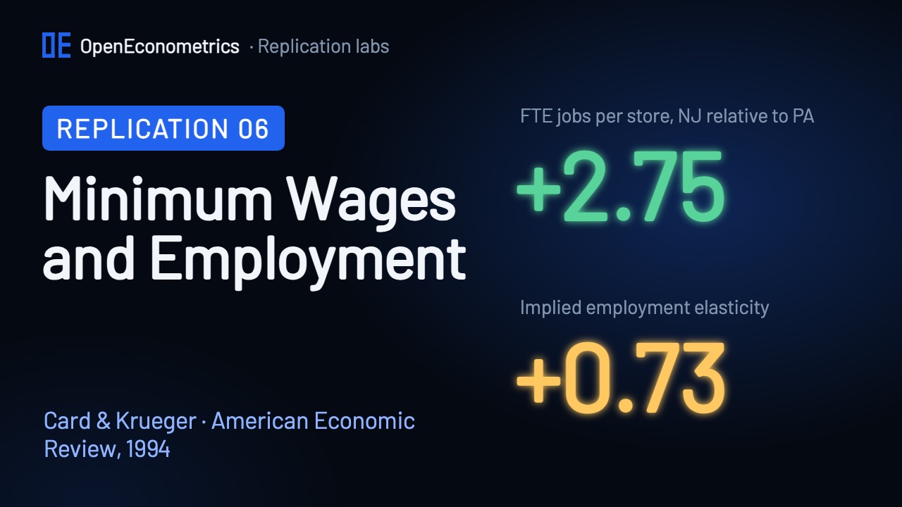
Pennsylvania stores started larger and lost employment; New Jersey stores started smaller and gained a little. Had New Jersey followed Pennsylvania's path, it would have ended at about 18.3 FTE per store. It ended 2.75 higher, about 13% of the average New Jersey store.

The key assumption is parallel trends: without the increase, New Jersey stores would have changed like Pennsylvania stores, on average. With two survey waves it cannot be tested, because there is no earlier period in which to see whether the two states moved together. The paper therefore adds a second comparison inside New Jersey: stores that already paid $5.00 or more were barely affected by the new minimum.

The regression version has one row per store. The change in FTE employment is regressed on a New Jersey dummy, whose coefficient is the difference in differences, with dummies for the chain and for company ownership as optional controls. The paper also measures treatment intensity with GAP, the raise the new law required as a share of the February starting wage w: (5.05 − w)/w for New Jersey stores paying less than $5.05, and 0 in Pennsylvania and for New Jersey stores already at $5.05 or more. A store paying $4.25 has a GAP of 0.80/4.25 = 0.1882; the mean among the New Jersey stores of the regression sample is 0.105 (the paper says 0.11).

The main results

Table 3 · mean FTE per store	Pennsylvania	New Jersey	NJ − PA	Paper, NJ − PA
1 · FTE before, all stores	23.33 (1.35)	20.44 (0.51)	−2.89 (1.44)	−2.89 (1.44)
2 · FTE after, all stores	21.17 (0.94)	21.03 (0.52)	−0.14 (1.08)	−0.14 (1.07)
3 · Change in mean FTE	−2.17 (1.23)	0.59 (0.47)	2.75 (1.31)	2.76 (1.36)
4 · Change, balanced sample	−2.28 (1.25)	0.47 (0.48)	2.75 (1.34)	2.75 (1.34)
5 · Change, temporarily closed = 0	−2.28 (1.25)	0.23 (0.49)	2.51 (1.35)	2.51 (1.35)

Pennsylvania stores went from 23.33 to 21.17 FTE, New Jersey stores from 20.44 to 21.03. The change in mean employment is −2.17 in Pennsylvania (printed −2.16, the difference of the two rounded means) and +0.59 in New Jersey, so the difference in differences is 2.75. The paper prints 2.76; the scorecard explains that hundredth. On the 384 stores with employment in both waves the difference in differences is 2.75 with a standard error of 1.34, exactly as printed, and counting the four temporarily closed stores as zero gives 2.51 (1.35). Employment did not fall in New Jersey relative to Pennsylvania.

Pennsylvania−2.28 (1.25)

NJ · paid $5.00 or more−2.16 (1.01)

NJ · paid $4.26–$4.990.71 (0.69)

NJ · paid $4.251.20 (0.82)

Table 3, row 4: stores with employment in both waves. The wage groups use the starting wage in February.

Inside New Jersey, stores that already paid $5.00 or more lost 2.16 FTE on the balanced sample, almost exactly Pennsylvania's 2.28. Stores paying $4.26 to $4.99 gained 0.71, and stores paying $4.25 gained 1.20 (printed 1.21, a rounding difference). Low-wage minus high-wage stores: 3.36 with a standard error of 1.30. The more a store had to raise its wage, the better its employment did, which is what the comparison with Pennsylvania says too.

Table 4 column	Regressor	Controls	Paper	This lab	SE of regression
(i)	New Jersey dummy	none	2.33 (1.19)	2.33 (1.19)	8.79
(ii)	New Jersey dummy	chain, ownership	2.30 (1.20)	2.30 (1.20)	8.78
(iii)	GAP	none	15.65 (6.08)	15.65 (6.08)	8.76
(iv)	GAP	chain, ownership	14.92 (6.21)	14.92 (6.21)	8.76
(v)	GAP	chain, ownership, region	11.91 (7.39)	11.98 (7.42)	8.75

Table 4 uses the 357 stores (290 in New Jersey, 67 in Pennsylvania) with employment and starting wages in both waves; the 6 stores that closed are included with zero employment. The New Jersey dummy is 2.33 (1.19), and 2.30 (1.20) with chain and ownership controls, which are jointly insignificant (p = 0.34). GAP gives 15.65 (6.08), and 14.92 (6.21) with the controls. All of these match the paper.

For a store that paid $4.25, the GAP coefficient implies 15.65 × 0.1882 = 2.95 more FTE, about 14% of the average New Jersey store's 20.44 FTE, as the paper's text says. Footnote 21 turns column (iv) into an employment elasticity with respect to the wage: 14.92 / 20.44 = 0.73. The competitive model predicts a negative number.

Specification tests

1 · Base specification2.30 (1.20)

2 · Temporarily closed counted as closed2.03 (1.22)

3 · FTE without managers2.34 (1.17)

4 · Part-time weighted 0.42.34 (1.20)

5 · Part-time weighted 0.62.27 (1.21)

6 · Without the shore stores2.59 (1.20)

7 · Interview-week dummies2.02 (1.20)

8 · Without hard-to-reach stores2.42 (1.29)

Change in FTE employment on the New Jersey dummy with chain and ownership controls. Rows 2 and 7 differ from the printed values; see the scorecard.

Table 5 changes one choice at a time and estimates the base model again. Rows 3 to 5 change how jobs are counted: without managers, or with part-timers weighted 0.4 or 0.6. Rows 2, 6 and 8 change the sample: the four temporarily closed stores count as closed, stores on the Jersey shore (35 in the survey), whose seasons may differ, are dropped, or stores that needed more than two call-backs in the first wave (70 in the survey) are dropped. Row 7 adds dummies for the week of the second interview, and row 9 weights the proportional change by each store's initial employment.

In levels the New Jersey effect is positive in every row, between 2.02 and 2.59 in this run. As a proportional change it is about 5% (0.05), and 0.13 (0.05) when stores are weighted by their size. Row 12 is a placebo: Pennsylvania stores get a "gap" to $5.05 that no law imposed, and its coefficient is −0.30 with a standard error of 22.00. Rows 10 and 11, towns around Newark and Camden, are selected by zip code, which the posted file does not contain, so the lab cannot reproduce them.

Modern checks

Two checks with the same data that the paper did not report. Table 4 uses conventional standard errors, which assume the same variance for every store, but the employment changes are more spread out in Pennsylvania (standard deviation 11.3) than in New Jersey (8.1). With heteroskedasticity-robust (HC1) standard errors, the New Jersey coefficient 2.33 has a standard error of 1.45 and a 95% interval from −0.53 to 5.18 (p = 0.11), so it is no longer significant at 5%; the interval still excludes a loss of more than about half an FTE per store. The GAP coefficient keeps a robust standard error of 6.17.

oe.didregress reproduces both differences of Table 3 as panel regressions on the 794 store-wave observations: with state and wave effects, 2.754 (1.307, clustered by store), the all-stores difference of row 3; with store fixed effects, 2.750 (1.338), the balanced-sample difference of row 4.

The scorecard

Target	Paper	This lab	Result
Table 3 · NJ − PA · balanced sample	2.75 (1.34)	2.7500 (1.3423)	✓ Match
Table 3 · NJ − PA · temporarily closed = 0	2.51 (1.35)	2.5092 (1.3460)	✓ Match
Table 3 · NJ − PA · all stores	2.76 (1.36)	2.7536 (1.3066)	Difference
Table 4 (i) · New Jersey dummy	2.33 (1.19)	2.3258 (1.1916)	✓ Match
Table 4 (ii) · New Jersey dummy	2.30 (1.20)	2.3039 (1.1955)	✓ Match
Table 4 (iii) · GAP	15.65 (6.08)	15.6529 (6.0802)	✓ Match
Table 4 (iv) · GAP	14.92 (6.21)	14.9157 (6.2053)	✓ Match
Table 4 (v) · GAP	11.91 (7.39)	11.9792 (7.4191)	Difference
Table 5 row 9 · proportional, weighted	0.13 (0.05)	0.1253 (0.0488)	✓ Match
Table 5 row 12 · Pennsylvania placebo	−0.30 (22.00)	−0.3044 (22.0034)	✓ Match
Tables 1 to 5 · every printed number	292 numbers	247 match · 15 rounding · 30 differ	Difference

Table	Numbers	Match	Rounding	Differ
Table 1 · Sample design and response	25	25	0	0
Table 2 · Means of key variables	88	82	1	5
Table 3 · Employment before and after	83	69	5	9
Table 4 · Reduced-form models	21	18	1	2
Table 5 · Specification tests	75	53	8	14
Tables 1 to 5	292	247	15	30

Of the 292 numbers printed in Tables 1 to 5 that the posted file can address, 247 match at the printed precision and 15 differ only in the last digit by a named rounding rule (10 by truncation, 3 as the difference of two printed entries, 2 by double rounding). 30 differ, and each one is kept with a diagnosis. Twenty statements with numbers in the text are checked as well: 14 match and 6 differ.

• Table 3, row 3 standard errors (8). The paper does not say how the standard error of a change in means allows for the same stores appearing in both waves. Clustering by store gives 1.31 for the difference in differences, against 1.36 printed. One common correlation of 0.45 between a store's two waves reproduces all eight printed standard errors, while the correlations in the data run from 0.48 to 0.66. That is consistent with an assumed correlation, not proof of the method, so the lab keeps its own values. The estimates are unaffected.
• Table 5, rows 3 to 5, proportional models (8). Footnote 18 and the authors' check.sas set the proportional change of a closed store to −1, and the lab follows them; so coded, the proportional models of rows 1, 2, 6, 8 and 9 match. In rows 3 to 5 they do not: row 3's GAP coefficient is 0.40 against 0.28 printed. Coding the six closed stores at −2, the value the formula itself gives when wave-2 employment is zero, reproduces all 12 printed proportional numbers of rows 3 to 5, such as 0.28 (0.34), and only 1 of 8 in rows 1 and 2. Those printed rows appear to have been computed without the footnote's rule.
• Table 5, row 7, interview-week dummies (5). The paper does not define its week dummies. With calendar weeks of the November survey and December as a fourth group, the lab gets 2.02 for New Jersey and 14.25 for GAP, against 2.27 and 15.79 printed; seven-day blocks from the first survey day give 2.25 and 15.75. No coding tried reproduces the whole row, although 3 of its 4 standard errors match.
• Data version (4). The file posted in 1997 has 283 New Jersey stores paying exactly $5.05 in November where the printed share implies 282, and gives a difference in differences of 2.7536 where a printed 2.76 needs at least 2.755.
• Table 4, column (v) (2). The table says the column controls for company ownership, but the authors' program leaves that dummy out, and the printed coefficient, 11.91 (7.39), is that model. With the dummy it is 11.98 (7.42); the printed standard error of the regression and p-value, 8.75 and 0.40, fit the model with it.
• Inside the paper (1) and unexplained (2). Tables 2 and 3 print different t statistics for the same wave-2 difference. A Table 2 t statistic and the New Jersey coefficient in Table 5, row 2 (2.03 against 2.20 printed) remain unexplained.

None of these changes the conclusion. Table 1, the first four columns of Table 4 and the balanced-sample difference in differences are reproduced exactly.

Where this replication stops

The comparison targets are the published tables. The authors' SAS output is not in the archive, so check.sas documents the variable construction and the Table 4 models, and the lab follows it. Table 1's first-wave sample frame and response rates, Table 5 rows 10 and 11 and the reliability ratios from the paper's 11 double interviews cannot be rebuilt from the posted file. Tables 6 to 8 and Figure 1 are outside the lab's scope; the wage distributions behind Figure 1 are exported and drawn in the lesson, but not compared with the figure.

The design has limits that no replication removes. With two waves, parallel trends cannot be tested. The horizon is eight months, the survey covers existing stores of four chains, and employment is reported by a manager over the phone. The study started a long debate: Neumark and Wascher (2000) re-examined the question with payroll records, and Card and Krueger (2000) replied with data from the Bureau of Labor Statistics, both in the American Economic Review. This lab uses none of those data and does not assess that debate.

Run it yourself

Watch the companion video above. The lab package will be published here. You will need the authors' files, which we do not redistribute because no licence terms are stated:

1. Run prepare_sources.py from the lab package. It downloads njmin.zip (23 kB: the survey data, the codebook, the two questionnaires and the authors' check.sas) and its readme from David Card's data page, and checks each file against its recorded SHA-256 fingerprint.
2. Open a Python document in OpenEconometrics, point the launcher at the lab, the authors' files and a new results folder, and press Run.

from lab import run_lab

result = run_lab(
    source_root=source_dir,
    output_dir=results_dir,
    display_callback=display,
)

Each column of Table 4 is one call:

fit = oe.regress(data=sample, y="dE", x=["gap", "bk", "kfc", "roys", "co_owned"])

The run writes reconciliation.csv, with every printed number next to the lab's result and a diagnosis for each difference.

The paper

David Card and Alan B. Krueger, "Minimum Wages and Employment: A Case Study of the Fast-Food Industry in New Jersey and Pennsylvania", American Economic Review 84(4), 772–793, September 1994. The published article has no registered DOI, so the "Read the paper" link above opens the NBER working paper of the same title. The lab's targets were transcribed from the scan of the journal pages that David Card links from his data page. Data: David Card's data page; no licence terms are stated. The paper and the authors' files keep their own rights; this page and the lab describe and recompute them.