Replication 01 · Economic Policy, 2025
The Simple Macroeconomics of AI
How much will AI raise productivity, GDP and wages in the United States over the next ten years?
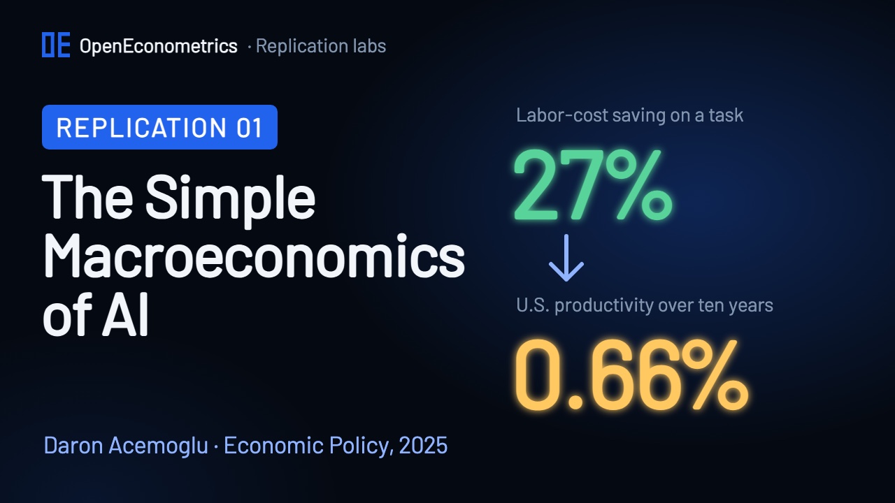
In two well-known experiments, an AI assistant cut the labor needed for a task by 27% on average. You might expect a productivity boom. Yet when Daron Acemoglu did the arithmetic for the United States, he arrived at about 0.66% more productivity, over ten years, not per year. This lab rebuilds that calculation from the author's own research files, follows it to GDP and to the wages of 500 groups of workers, and checks every published number against ours.
A big saving on a small slice
Imagine an economy that produces $100 of output, of which $10 pays for writing reports. If a new tool makes reports 20% cheaper, the economy saves $2: a productivity gain of 2%. This is the idea behind Hulten's theorem. A small improvement in one activity raises aggregate productivity by that activity's share of the economy times its cost saving.
Acemoglu applies the same logic to AI. The change in total factor productivity (TFP) is approximately the GDP share of the tasks AI affects, times the average cost saving on those tasks. So the paper has to measure two things: how big the slice is, and how much AI saves there.
The four numbers behind the headline
- Exposure. Using task scores from Eloundou and coauthors (2023), weighted by each occupation's share of the U.S. wage bill, about 20% of the wage bill is exposed to AI. Our reconstruction from the author's files gives 19.98%.
- Worth automating. Following Svanberg and coauthors (2024), only 23% of exposed work is economically worthwhile to automate. That leaves 4.6% of the economy affected.
- Labor-cost saving. The average of two experiments, on professional writing and customer support, is a 27% saving in labor cost.
- Labor share. Labor is only part of production costs. In the exposed industries it is 53.56% (the paper's main text prints 53.5%), so the total cost saving is 14.46%.
4.60% affected × 14.46% cost saving = 0.6645% TFP over ten years
Exposure is far from even. Averaged over the jobs in each industry, it is about a third in finance, insurance and real estate, and around one in ten in construction and agriculture.
Easy tasks and hard tasks
The experiments behind the 27% studied tasks with a clear goal and an outcome that is easy to check. Acemoglu calls these easy tasks. Hard tasks depend on context and judgment, and success is hard to judge, so the paper assumes a labor saving of only 7% there. A classifier sorts exposed tasks into the two groups: 72.6% of the exposed wage bill turns out to be easy.
Applying the two savings separately lowers the ten-year TFP gain from 0.66% to 0.53%, about a fifth less.
Bars are drawn against 1%: every scenario stays below it.
Raising the share worth automating from 23% to 30% gives about 0.87%. Adding a third experiment, on software developers, gives about 0.89%. These are scenarios, not forecasts with confidence intervals.
From productivity to GDP
When production becomes more efficient, it pays to invest in more capital. If capital grows to keep the capital-to-output ratio constant, GDP rises by the TFP gain divided by one minus the capital share. With a capital share of 43%, the multiplier is about 1.75.
For the easy-and-hard scenario we get 0.93%, exactly as printed. For the baseline our full-precision result is 1.1657%, which rounds to 1.17%; the paper prints 1.16%. Rounding TFP to 0.66% first and dividing by 0.57 gives 1.158, which explains the printed digit. We keep the full-precision value and record the difference.
Who gains and who loses
For wages, the paper uses a task-based general-equilibrium model with 500 groups of workers, defined by gender, age, education, race and birthplace, across 49 industries. Workers in automated tasks are displaced, cheaper production raises demand, industries grow and shrink, and displaced workers compete for other tasks. In the full model, GDP rises by 1.56% over the decade.
| Education | Work affected by AI | Direct wage effect | Total wage effect |
|---|---|---|---|
| Less than high school | 3.18% | −3.23% | +1.57% |
| High school | 4.64% | −6.17% | +1.06% |
| Some college | 4.94% | −6.76% | +1.39% |
| Bachelor's degree | 5.23% | −7.33% | +0.60% |
| Postgraduate | 4.05% | −4.98% | +0.98% |
| Average worker | 4.62% | −6.12% | +1.01% |
For the average worker, AI affects 4.6% of their work. The direct effect of losing those tasks is −6.1%, but once productivity and industry shifts feed back, the total wage effect is a gain of about 1%.
AI also differs from the automation of the past. Between 1980 and 2016, task displacement from automation was about 27% for workers with a high-school degree or less and about 3% for postgraduates. AI's reach is smaller and spread more evenly.
Automation, 1980–2016: task displacement (%)AI: share of work affected (%)
On average, men gain about 1.7% and women lose about 0.3%: in these data, AI affects 5.4% of women's work against 3.9% of men's. Labor's share of income falls by 0.31 percentage points, while the standard deviation of log wages across the 500 groups barely moves, from 0.35 to 0.36. In this model, AI widens the gap between capital and labor more than the gaps between workers.
The scorecard
| Target | Paper | This lab | Result |
|---|---|---|---|
| TFP gain · baseline | 0.66% | 0.6645% | ✓ Match |
| TFP gain · easy and hard tasks | 0.53% | 0.5295% | ✓ Match |
| GDP · easy and hard tasks | 0.93% | 0.9289% | ✓ Match |
| GDP · baseline | 1.16% | 1.1657% | Rounding |
| GDP · full wage model | 1.56% | 1.5607% | ✓ Match |
| Table 1 · 50 numbers | 49 of 50 match | ✓ Match | |
| Bachelor’s · historical exposure | 0.0684 | 0.0683 | Difference |
Both TFP headlines and the easy-and-hard GDP figure match. The baseline GDP figure differs in its last digit for the rounding reason above. In Table 1, 49 of 50 numbers match at the printed precision; the exception is the historical exposure of bachelor's-degree workers, 0.0683 against a printed 0.0684. The wage model's saved results for all 500 groups agree with the author's archived output to about 17 decimal places.
Where this replication stops
The lab rebuilds the wage-bill weights, the industry labor shares, every macro scenario, the full wage model, Table 1 and the paper's figures. It takes four things as given:
- the task-level exposure weights, which are not in the public archive, so the lab starts from the author's occupation-level exposure numbers;
- the cleaning of the census microdata;
- the topic model and the easy/hard classifier, whose saved results are used as inputs;
- the calibrated parameters of the wage model, which are not re-estimated.
It is therefore a complete rebuild of the paper's calculations from the author's prepared inputs, not a replication from raw data.
Run it yourself
The lab package and the companion video will be published here. You will need the author's replication archive, which we never redistribute:
- Download the replication files for The Simple Macroeconomics of AI from Daron Acemoglu's data archive at MIT.
- Run
prepare_sources.pyfrom the lab package. It extracts the 97 files the lab needs and checks each one against its recorded SHA-256 fingerprint. - Open a Python document in OpenEconometrics, point the launcher at the lab, the author's files and a new results folder, and press Run.
from lab import run_lab

result = run_lab(
    source_root=source_dir,
    output_dir=results_dir,
    display_callback=display,
)
The run displays the macro summary, Table 1 and two interactive charts, and writes reconciliation.csv with every published number next to the lab's result.
The paper
Daron Acemoglu, "The Simple Macroeconomics of AI", Economic Policy 40(121), 13–58, 2025. doi:10.1093/epolic/eiae042. The paper, the author's data and third-party code keep their own rights; this page and the lab describe and recompute them.