Econometrics · Lab 15 of 20
Before and After a Policy Reform
Difference-in-Differences
Can an employment program work even when the regions receiving it still have lower employment afterward? This lab evaluates a fictional regional training subsidy introduced in 2018. Its purpose is to separate the policy comparison from the assumptions that make that comparison causal.
All observations are original synthetic data supplied in policy_panel.xlsx. No people, regions, or policy outcomes are represented. The reported numbers are actual OpenEconometrics estimates from that simulated dataset, not evidence about an actual subsidy. A pre-treatment diagnostic raises a warning that we will interpret alongside the policy estimate.
Learning goals
By the end, you should be able to compute DiD from four means, connect it to a regression interaction and a model with region and year effects, interpret a clustered confidence interval, and explain why a promising coefficient or a pre-trends test cannot establish policy identification alone.
Topic alignment: Stock and Watson, Introduction to Econometrics, fourth edition, Chapters 10 (panel data) and 13 (experiments and quasi-experiments). This is an original teaching exercise; it reproduces no textbook problem or dataset.
1. Ask the right policy question
Thirty regions receive the subsidy and thirty never receive it during the sample. We observe every region annually from 2015 through 2020; all treated regions begin treatment in 2018 and remain treated. Each observation is one region-year, not an individual worker.
The target is the average policy effect in the treated regions over 2018–2020, measured in employment percentage points. The comparison is with employment in those same regions, in those same years, had the subsidy not existed. That counterfactual is normally unobserved. The never-treated regions supply a candidate comparison for the change that would otherwise have occurred.
The fictional administrative rule targets regions with lower underlying employment levels. Therefore a lower post-policy employment level in treated regions does not, on its own, show that the policy reduced employment. A rise within treated regions does not isolate the effect either: national employment conditions may improve at the same time.
2. Understand the data before fitting
The balanced panel has 360 observations, 60 regions, three pre-policy years, and three post-policy years. No observations are missing and no weights are used. Each region receives equal weight; this is not a population-weighted national employment estimate.
| Variable | Definition | Unit / coding |
|---|---|---|
region | Independent policy and uncertainty unit | Integer 0–59 |
year | Observation year | 2015–2020 |
treated | Region ever receives the subsidy | 1 for regions 0–29; otherwise 0 |
post | Policy is available during this year | 1 from 2018 onward |
treated_post | Actual treatment exposure | treated * post |
employment_rate | Observed synthetic employment rate | Percent of working-age population |
employment_no_policy | Simulated untreated potential outcome | Teaching oracle only; excluded from estimation |
The prepared observations follow this synthetic design: untreated employment contains a region intercept, a six-point lower level for the treated group, a common 1.2-point annual trend, common year shocks, and region-specific errors with AR(1) persistence 0.65. Errors are independent across regions. Treatment adds exactly 3.0 percentage points to every treated post-policy observation. Thus expected untreated trends are parallel by construction; realized sample paths still fluctuate.
The known simulated counterfactual helps us learn what the estimator does. Do not include employment_no_policy as a control or assume that it exists in an empirical dataset.
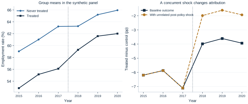
Read the figure in two stages: compare pre-policy changes first, then examine the change in the gap after 2018. Identical starting levels are not required for DiD. Similar-looking pre-period paths are useful descriptive evidence but do not identify the missing post-period counterfactual.
3. Compute the four-cell comparison
Let and denote the treated group's means over the three pre- and three post-policy years. Define the control means similarly. The estimator is
Download policy_panel.xlsx and lab.py. In OpenEconometrics, import the workbook without changing its filename, then open lab.py in a Python document and run the complete file. The workbook's first sheet, Data, contains the observations; Dictionary explains the variables and units.
The script reads the prepared panel, fits the models, performs the checks, and displays the four-cell table, the main model, the gap chart, and the concurrent-shock model. Everyone using the supplied workbook starts from the same observations and obtains the same reported results.
In ordinary Python, keep the workbook beside lab.py and run python lab.py from an environment where OpenEconometrics is installed. To read a workbook from another folder, use from lab import run_lab, then call run_lab(data_path="/path/to/policy_panel.xlsx"). The script writes no exports unless an output directory is explicitly supplied.
After running the complete file, explore the same data interactively:
data = load_data()
means = data.groupby(["treated", "post"]).employment_rate.mean()
did_by_hand = (
    means[1, 1] - means[1, 0]
    - (means[0, 1] - means[0, 0])
)
print(did_by_hand)| Group | Pre-policy mean | Post-policy mean | Change |
|---|---|---|---|
| Never treated | 61.084 | 64.803 | 3.719 |
| Treated | 54.691 | 60.959 | 6.268 |
Thus percentage points, using the unrounded values in code. The treated-only before–after change is 6.268 points and the post-only treated-minus-control gap is −3.844 points. These comparisons answer different questions. DiD subtracts the control change to estimate the policy contrast under its identifying assumptions.
4. Connect the arithmetic to regression
The two-way fixed-effects specification is
Region effects absorb permanent differences in levels; year effects absorb shocks common to all regions in a year. The coefficient on is the DiD contrast in this balanced common-adoption design. We have one adoption date and a constant simulated treatment effect. This lab makes no claim about interpreting ordinary two-way fixed effects under staggered adoption with heterogeneous effects.
did = oe.didregress(
    data=data,
    y="employment_rate",
    treatment="treated_post",
    group="region",
    time="year",
    covariance="cluster",
    cluster="region",
    missing="raise",
    alpha=0.05,
)
print(did.summary())
Pass actual exposure treated_post to treatment, not the time-invariant treated indicator. Region effects would absorb the latter. The lab also fits the saturated regression employment_rate ~ treated + post + treated_post on the identical observations. Its interaction coefficient, the native DiD coefficient, and the four-cell calculation agree to numerical precision here. Their equality relies on this balanced, equally weighted design; do not generalize the shortcut to every panel or adjusted specification.
5. Interpret the estimate and uncertainty
| Quantity | Executed result |
|---|---|
| DiD estimate | 2.549 percentage points |
| Region-clustered standard error | 0.438 |
| 95% confidence interval | [1.673, 3.426] percentage points |
| Two-sided p-value | 0.000000257 |
| Inference distribution | Student , 59 degrees of freedom |
| Known simulated policy effect | 3.000 percentage points |
The estimated treated-region improvement exceeds the comparison-region improvement by 2.549 points. This is not a 2.549% proportional increase. Under the maintained design and uncertainty assumptions, the interval quantifies sampling uncertainty about that contrast. It includes the true simulated three-point effect. A confidence interval does not assign a probability to the identifying assumptions being correct.
Clustering is at the region, where policy varies and errors persist across years. The six observations from one region are not six independent policy experiments. Serial correlation can materially distort DiD inference when ignored; see Bertrand, Duflo, and Mullainathan. There are 60 independent clusters in this illustration, rather than only two clusters labeled “treated” and “control.”
The native estimator uses the small-sample multiplier
and inference. Here counts one treatment slope and six time effects; region effects nested in region clusters are excluded from that correction. The script independently demeans the balanced panel and calculates the scalar cluster sandwich. Its coefficient and standard error match the native result. The saturated two-by-two regression uses a different finite-sample parameter count; equality of coefficients is not a claim that every reported standard error must be identical.
6. Identification: make the assumptions explicit
Parallel trends concerns untreated potential outcomes, not observed post-treatment outcomes:
For a causal interpretation, also argue that treatment was not anticipated, comparison regions were not affected through spillovers, outcome measurement and sample composition remain comparable, and no other treated-specific change coincided with the subsidy. In this synthetic panel, stable composition and independent regions are explicit design choices. In an empirical project they would require substantive evidence.
The native linear pre-trend test returns p = 0.0712, while the joint pre-treatment-leads test returns p = 0.0098. At a 5% threshold the first does not reject and the second does reject. The tests ask different questions. The joint result is a warning that deserves inspection; it cannot be discarded because the headline estimate is attractive. Even a correctly specified population model can produce an unusually large sample diagnostic. Conversely, non-rejection would not establish parallel counterfactual trends or rule out a post-treatment shock. The supplied sample is retained even when its diagnostics are not reassuring. See Roth's discussion of pre-testing.
Now add an unrelated two-point employment boost that occurs only in treated regions, beginning in 2018:
contaminated = data.copy()
contaminated["employment_rate"] += 2.0 * contaminated.treated_post
The full script refits the model on this outcome. The coefficient becomes 4.549, with the same 0.438 standard error and interval [3.673, 5.426]. The pre-treatment data and diagnostic p-values are unchanged. The known policy effect remains three points; the added shock is not part of the subsidy. DiD cannot distinguish the two perfectly coincident changes. Better precision about the combined change cannot repair this identification failure.
Follow the counterfactual through the arithmetic
Start with the treated regions' pre-policy mean. Under parallel untreated trends, add the control regions' average change. The resulting level is the treated regions' predicted post-policy mean without the subsidy. Subtract that counterfactual from their observed post-policy mean. This produces the same DiD as subtracting the two changes, but makes the missing comparison more visible:
The first expression is a constructed counterfactual, not an observed group mean. It is credible only if the comparison group's change is informative about the treated regions' untreated change. A permanent difference in levels need not violate that condition. A different underlying trend, spillover or treated-only concurrent reform can violate it even when the pre-policy levels look similar.
Understand what one cluster contributes
The sample contains six annual observations from each region. A local shock can persist across those years, so six observations from one region are not equivalent to six independent regions. Region clustering forms a score contribution for each region and allows dependence among that region's yearly disturbances. The information supporting inference comes from 60 clusters, including 30 treated clusters, rather than 360 unrelated treatment assignments.
This explains why the reported interval uses 59 inference degrees of freedom. It does not make 60 a universal threshold for reliable inference. An uneven design with very few treated regions, a dominant region, or shocks correlated across regions could still demand additional care. Matching the clustering unit to the policy and disturbance structure is a design decision, not a search for the covariance method that gives the smallest standard error.
A precise estimate can still answer the wrong causal question
The concurrent-shock example has a clear statistical comparison: the treated outcome rises by an additional two points exactly when treatment starts. The estimator correctly incorporates that additional change. The identification problem is that the observed outcome does not label which part was produced by the subsidy and which part by the other event.
A narrow interval around the combined change would describe statistical precision conditional on the maintained model. It would not distinguish the two mechanisms. More observations of the same confounded pattern can make the combined effect more precise while leaving the attribution problem intact. Policy documents, implementation dates, alternative outcomes and credible comparison groups can therefore matter as much as a larger sample. The regression organizes a comparison; the research design explains why that comparison should identify the effect of interest.
Student exercises
- Calculate the DiD from the four displayed means. Explain why using rounded values can differ slightly from the script.
- Write one sentence interpreting the 2.549 coefficient and one explaining why the −3.844 post-policy gap is not the same estimand.
- Fit the saturated interaction model and locate
treated_post. Why cantreatedandpostappear there, while they are absorbed by region and time effects in the native model? - Replace clustered covariance with
covariance="HC1"inoe.didregress. Does the coefficient change? Which dependence assumption changes? Do not choose an uncertainty method because its p-value is smaller. - Explain what the two pre-treatment diagnostics can and cannot tell us. Would both p-values above 0.05 eliminate concern about the concurrent shock?
- Read the concurrent-shock estimate as a hypothetical policy memo. Identify the additional evidence you would need before attributing it to the subsidy.