Econometrics · Lab 18 of 20
Accounting for Persistent Shocks
Serial correlation and HAC inference.
A firm increases advertising in one quarter and keeps much of that spending level in the next. Demand shocks also persist: a favorable quarter is often followed by another favorable quarter. A regression can still estimate the advertising–sales relationship, but observations close together in time do not provide the same uncertainty information as independent draws.
This lab separates two tasks that are often conflated: fitting an OLS coefficient and estimating its sampling uncertainty. We fit exactly the same model on exactly the same observations using HC1 and two declared HAC specifications. The coefficient does not change. Its standard error and confidence interval do change because the covariance calculations allow different dependence patterns.
The advertising and sales series are original synthetic data, not company records. They are supplied in advertising_and_sales.xlsx. lab.py reads these observations, performs the native OpenEconometrics fits, and presents the calendar-aware HAC comparison. The results illustrate inference under a specified process rather than an empirical estimate of advertising returns.
1. Explain why nearby quarters can contain overlapping information
Write the regression as
If errors are independent across periods, the variance of a sum of regression scores depends on each period's variance. If errors and regressors are persistent, cross-period covariance terms also matter. A favorable demand shock lasting several quarters should not be counted as several independent surprises about the slope.
HC1 allows the variance of to differ across observations, but it does not include nonzero cross-period covariance terms. HAC stands for heteroskedasticity and autocorrelation consistent. It estimates a covariance matrix that can accommodate both changing variance and short-range serial dependence under appropriate regularity conditions.
The relevant object is the regression score , with including the intercept, not simply the error series in isolation. Persistence in both the regressor and errors can make the score covariance important for the slope. Correcting only for heteroskedasticity may therefore leave substantial uncertainty unaccounted for.
Serial correlation does not automatically bias the OLS coefficient. Under a suitable exogeneity condition, the point estimator can remain consistent while its conventional covariance formula fails. If the regressor is correlated with the error, however, changing the covariance estimator does not solve that endogeneity problem.
For an AR(1) error with persistence and innovation variance , the stationary error variance is and its lag- covariance is that variance multiplied by . Positive persistence therefore creates many positive covariance terms. The uncertainty of an average can be much larger than a calculation that counts only each quarter's individual variance. For a regression slope, the same intuition applies through the score products, although their signs and magnitudes also depend on the regressor path. This is why examining only the number of rows can give a misleading impression of how much independent information a time series contains.
2. Inspect the original synthetic process and calendar
The prepared series follow independent innovation sequences and persistent processes:
where the innovation standard deviations are 0.5 and 1.0 respectively. The outcome is
One hundred initial simulated periods are discarded before the 200-period teaching series is retained. This reduces the influence of initializing both deviations at zero. The two innovation streams are independent, so the generator does not deliberately create endogeneity between advertising and demand shocks.
| Variable | Definition | Unit |
|---|---|---|
quarter | Original integer calendar position | 1–200 |
advertising | Synthetic quarterly advertising expenditure | Ten thousand currency units |
sales | Synthetic quarterly quantity sold | Thousand units |
Three known unavailable quarters—40, 41, and 95—are excluded explicitly. The resulting sample contains 197 observations, and all fits use those same observations. The original quarter labels are preserved. The script does not silently compress the series into a gap-free calendar of length 197.
This distinction affects HAC. Observed quarters 39 and 42 are three calendar periods apart even though their rows become adjacent after exclusions. A procedure that treated them as lag one would estimate a different covariance matrix. Missing-data handling is therefore part of the statistical specification, not just file preparation.
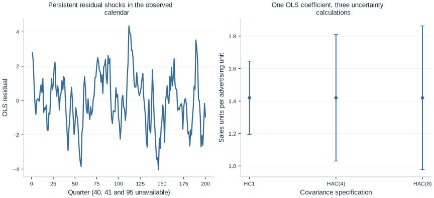
The residual panel shows runs of positive and negative disturbances. The interval panel compares the same slope under three covariance choices. Read the calendar axis literally: a line joining observed values does not mean outcomes were observed or imputed in the excluded quarters.
3. Run one model with three covariance choices
Download advertising_and_sales.xlsx and lab.py. In OpenEconometrics, import the workbook without changing its filename, then open lab.py in a Python document and run the complete file. The workbook's first sheet, Data, contains the observations; Dictionary explains the variables and units.
The script reads the observed calendar without renumbering its gaps. The application displays the main HAC model, a comparison table, and the residual chart. Everyone using the supplied workbook starts from the same observations and obtains the same reported results.
In ordinary Python, keep the workbook beside lab.py and run python lab.py from an environment where OpenEconometrics is installed. To read a workbook from another folder, use from lab import run_lab, then call run_lab(data_path="/path/to/advertising_and_sales.xlsx"). The script writes no exports unless an output directory is explicitly supplied.
The HC1 fit establishes the point model and one uncertainty comparison:
data = load_data()
hc1 = oe.ols(
    data=data, y="sales", x=["advertising"],
    covariance="HC1", missing="raise", device="cpu",
)
The main HAC fit makes the calendar and lag choice explicit:
hac4 = oe.ols(
    data=data, y="sales", x=["advertising"],
    covariance="hac",
    time="quarter",
    lags=4,
    kernel="bartlett",
    missing="raise",
    device="cpu",
)
print(hac4.summary())
The complete script also fits the same model with lags=8. No outcome, regressor, weight, or sample changes across these specifications. Hence each model reports the same fitted line:
In the declared units, an additional ten thousand currency units of quarterly advertising is associated with about 1.420 thousand additional sales units. That is a quantity association, not a monetary profit calculation. Revenue, production costs, campaign pricing, and a causal design would be needed for a return-on-investment claim.
4. Read the uncertainty comparison accurately
| Covariance calculation | Slope | Standard error | 95% interval |
|---|---|---|---|
| HC1 | 1.420132 | 0.114609 | [1.194100, 1.646164] |
| Bartlett HAC, 4 lags | 1.420132 | 0.197559 | [1.030506, 1.809759] |
| Bartlett HAC, 8 lags | 1.420132 | 0.224602 | [0.977171, 1.863093] |
The main HAC standard error is substantially larger than HC1's in this sample. Including eight lags produces a wider interval still. The known synthetic slope, 1.4, lies inside all three intervals; that single fact does not establish which covariance estimator would have appropriate repeated-sample coverage.
HAC standard errors are not guaranteed to exceed HC1 standard errors, nor must they grow monotonically when the lag choice changes. Cross-covariance terms can be positive or negative, and the kernel weights change with the lag bandwidth. The ordering here follows this realized persistent process, not a universal rule about “robustness.”
OpenEconometrics reports Student t reference inference with 195 degrees of freedom, equal to 197 observations minus two fitted coefficients. For HAC, this is a reporting convention and finite-sample approximation; it does not make HAC intervals exact finite-sample intervals for every serially dependent process. HAC consistency relies on large-sample arguments and suitable dependence and bandwidth behavior.
5. Build intuition for the Bartlett sandwich
Let , let be the OLS residual, and define the estimated score . The HAC meat includes contemporaneous and lagged score products:
For , the lag weights are 0.8, 0.6, 0.4, and 0.2. Dependence closer in time receives more weight. Products beyond lag four are not included in this declared Bartlett calculation. Setting four lags does not assert that the true error correlation becomes exactly zero after four quarters.
The reported covariance matrix is
The outer matrices translate variation in the scores into variation in fitted coefficients. The multiplier is the finite-sample correction used here. The same fitted residuals enter every covariance comparison, so the change in uncertainty comes from which score products are included and how they are weighted. Including serial products changes the sampling-variance estimate without changing the least-squares objective or its minimizing coefficients.
An important implementation detail is the inner sum. It uses pairs whose actual calendar distance is . For lag one, quarter 39 is not paired with quarter 42. For lag three, it is. Dropping a row and relabeling the remaining rows would change that set of pairs and therefore change the question asked by the covariance calculation.
6. Choose a dependence specification from the problem
The lag bandwidth balances two considerations. Including more covariance terms can represent longer-lived dependence, while estimating many noisy terms can make the covariance estimate unstable. The correct choice depends on sampling frequency, process persistence, sample length, and the inferential goal. There is no single lag count that works for every quarterly series.
Here four and eight lags are declared examples. A substantive application might motivate a lag range from business cycles, contract renewal periods, or known reporting patterns, and examine sensitivity over a justified set. An automatic bandwidth rule is another possibility, but it too embodies assumptions and should be recorded. Selecting the lag count because it creates the preferred significance result is not a defensible selection strategy.
Inspecting residual plots helps reveal persistence and unusual episodes. It does not replace reasoning about how regressors, errors, and calendar units are generated. A residual correlation that appears small in one sample may still matter for a particular contrast, and an isolated plot cannot diagnose every failure of the model.
The excluded quarters are a deliberately transparent teaching choice. In real data, missing sales could reflect a reporting failure correlated with unusually bad outcomes. Preserving calendar gaps would then be necessary but insufficient: the selection mechanism itself could threaten the analysis. Accurate time indexing does not make the observed sample representative.
7. Know the limits of changing the covariance estimator
HAC does not change the fitted conditional mean. If the slope is biased because advertising responds to an unobserved demand forecast, HAC leaves that problem in place. If the true mean has a neglected seasonal pattern or a structural break, a different covariance matrix may not provide the most useful model. If the level series contain unit roots and produce a spurious regression, simply requesting HAC is not a complete treatment of that nonstationary setting.
There is also a difference between correcting inference and modeling dynamics. A dynamic model might include lagged outcomes or specify an autoregressive error process for forecasting or efficiency. HAC allows a broader class of dependence when estimating uncertainty for a chosen regression, without requiring us to fit the exact AR(1) generator. The choice between these goals should follow the research question.
Finally, remember the unit of independence. This example is one time series, with dependence organized by temporal distance. A multi-region panel with common shocks may call for a different covariance design, such as appropriate clustering or a panel-specific dependence method. Copying a single-series HAC call onto a panel with repeated quarter labels would not preserve this specification.
8. Communicate the result
The publication LaTeX table presents the three covariance specifications together. Keep the identical point model and sample visible so that a reader can attribute the changing intervals to the uncertainty calculation rather than an undisclosed change in regressors or observations.
A clear result paragraph states the regression, units, 197-observation sample, excluded calendar periods, Bartlett kernel, four-lag choice, and interval. It also distinguishes the estimated association from a causal or commercial return claim. Report the eight-lag comparison as sensitivity rather than silently choosing whichever interval is most convenient.
9. Questions for your analysis
- Explain why serial correlation can affect uncertainty without necessarily changing the consistency of OLS under exogeneity. What additional problem arises if advertising is correlated with demand shocks?
- Explain the different dependence assumptions behind HC1 and HAC. Why is the score covariance relevant to the slope, not just the residual variance?
- Reconstruct the Bartlett weights for four and eight lags. Explain the role of the finite-sample multiplier in the displayed sandwich.
- Identify which lag pairs would be incorrectly created if quarters 40, 41, and 95 were dropped and the remaining observations were renumbered.
- Interpret the main slope and confidence interval using the declared advertising and sales units. Explain why the estimate is not a profit rate.
- Discuss the bandwidth comparison without assuming HAC standard errors must always be larger or monotone in the lag count.
- Describe two model or design failures that HAC cannot repair, and propose evidence or analysis that would address each one.