Econometrics · Lab 19 of 20
Forecasting Inflation Without Looking Ahead
Autoregressive models, time-ordered evaluation and forecast errors.
Suppose the latest available inflation observation is quarter 160 and a planning team wants a forecast path for the next twenty quarters. We can fit an autoregression using the history available at that date. We cannot use quarter 170's realized inflation to improve a forecast supposedly made ten quarters earlier.
This lab makes that information boundary explicit. It estimates a native OpenEconometrics AR(1) model on quarters 1–160, forecasts quarters 161–180 from a single fixed origin, and evaluates the predictions on the untouched future observations. Two simple benchmarks use the identical origin and evaluation window. The geometric forecast formula explains how a persistent shock fades and how new innovations create future uncertainty.
The inflation series is original synthetic data. It is not a country's inflation history and is not an economic forecast for a real economy. All 180 observations are supplied in forecast_series.xlsx. They follow a declared stationary process. All reported estimates and losses come from executing lab.py on that workbook.
1. Define the forecast before choosing the model
Our target is a path of future inflation values, measured in percent, over horizons from origin . The information set contains only observations through . The desired conditional-mean forecast is
under the fitted forecasting model. The notation after the vertical bar is essential: every point in this path uses the same information set.
This is one twenty-step dynamic forecast, not twenty forecasts repeatedly updated with newly observed outcomes. In a rolling one-step exercise, the forecast for quarter 162 could use quarter 161's actual value. In this fixed origin exercise it cannot. The tasks have different information and error structures, so their loss statistics should not be compared as though they were interchangeable.
The model is chosen as a transparent teaching specification before examining held-out loss. We do not select among dozens of lag orders using the same twenty observations that we later describe as an untouched test set. If model selection were required, it would need a separate training/validation design or an explicitly nested time-ordered procedure.
2. Understand the supplied series and split
The supplied synthetic series follows
The first 200 simulated periods are discarded. We then retain 180 consecutive observations. The known long-run mean is 2.5%, the persistence parameter is 0.75, and the innovation standard deviation is 0.45 percentage points. The analyst fits the model without supplying those true parameters.
| Data component | Calendar range | Observations | Role |
|---|---|---|---|
| Training history | 1–160 | 160 | Estimate every model parameter |
| Forecast origin | 160 | Latest available observation | Initialize the prediction path |
| Held-out outcomes | 161–180 | 20 | Evaluate previously fixed forecasts |
The variables are quarter, a consecutive integer time index, and inflation, a synthetic quarterly rate expressed in percent. A change from 2.5 to 3.0 is half a percentage point. No external predictors, revisions, seasonal adjustment, or survey expectations enter this example.
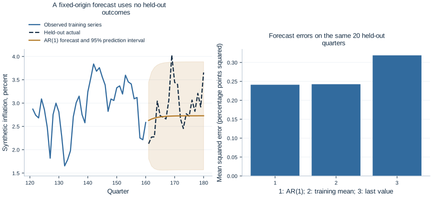
The observed training path stops at the origin. The forecast path approaches the estimated long-run mean; the held-out actual path continues to receive new shocks. Forecasting does not predict the realized future innovations. The shaded interval describes model-based outcome uncertainty, not a range chosen after seeing where the future observations happened to fall.
3. Fit a native AR(1) using training data only
Download forecast_series.xlsx and lab.py. In OpenEconometrics, import the workbook without changing its filename, then open lab.py in a Python document and run the complete file. The workbook's first sheet, Data, contains the observations; Dictionary explains the variables and units.
The script preserves the workbook order, fits only quarters 1–160, and reserves quarters 161–180 for evaluation. It displays the fitted model, the twenty-row evaluation table, a native forecast chart, and the benchmark loss table. Everyone using the supplied workbook starts from the same observations and obtains the same reported results.
In ordinary Python, keep the workbook beside lab.py and run python lab.py from an environment where OpenEconometrics is installed. To read a workbook from another folder, use from lab import run_lab, then call run_lab(data_path="/path/to/forecast_series.xlsx"). The script writes no exports unless an output directory is explicitly supplied.
The important split occurs before estimation:
data = load_data()
train = data.iloc[:160].copy()
test = data.iloc[160:].copy()

model = oe.arima(
    data=train,
    y="inflation",
    order=(1, 0, 0),
    time="quarter",
    method="ml",
    covariance="nonrobust",
    missing="raise",
    alpha=0.05,
    ljung_lags=8,
)
print(model.summary())
The order (1, 0, 0) specifies one autoregressive lag, no differencing, and no moving-average term. Exact Gaussian maximum likelihood estimates the stationary AR model; the requested covariance uses observed-information inference. This is not the same estimation objective as simply running a conditional regression and dropping the first observation.
OpenEconometrics parameterizes this model as
Its reported Intercept is the long-run mean , not the recursion constant in . Those parameters satisfy . Confusing them would give the wrong forecast even if the estimated AR coefficient were read correctly.
| Fitted parameter | Estimate | Standard error |
|---|---|---|
Long-run mean, Intercept | 2.728028 | 0.110624 |
Persistence, ARMA:L1.ar | 0.704108 | 0.056795 |
Innovation SD, /sigma | 0.419674 | 0.023461 |
These estimates differ from the generator's true values because only one finite training history is available. Knowing the simulation parameters is useful for interpretation, but replacing estimated parameters with them would turn this into a different forecasting exercise.
4. Forecast without feeding future actual values back into the model
The native call starts from the fitted result's saved final state:
forecasts = oe.forecast(model, steps=20, alpha=0.05)
print(forecasts)
The output calendar begins at 161 and ends at 180. No held-out outcome is passed to the forecast call. For a stationary AR(1), the point path can also be written directly as
At the origin, actual inflation is 2.585473%, below the estimated mean 2.728028%. The one-step forecast is 2.627654%; the twenty-step forecast is 2.727900%. The initial deviation decays geometrically because . The forecast can move toward the mean while actual future inflation moves elsewhere, because new shocks occur after the origin.
This mean-reverting path is not a forecast of central-bank actions or a structural account of inflation. It is the model's statistical conditional mean, based only on the past inflation series. An autoregressive coefficient does not identify a causal policy response.
5. Distinguish a prediction interval from parameter uncertainty
For the fitted AR(1), the future innovation contribution is
when fitted parameters are treated as fixed. Its variance is
The native forecast standard error is . It is 0.419674 at horizon one and 0.591012 at horizon twenty. For a stationary AR(1), the variance approaches rather than increasing without bound.
The normal 95% prediction interval is the point forecast plus or minus approximately . At horizon one the interval is [1.805109%, 3.450199%]; at horizon twenty it is [1.569537%, 3.886263%]. These intervals concern future inflation outcomes, which receive new innovations. They are not confidence intervals for the long-run mean or the AR coefficient.
The native interval here includes innovation uncertainty only. It excludes uncertainty about the estimated parameters, model selection, structural change, and a potentially incorrect innovation distribution. The relatively short training history means those omitted sources can matter. Labeling the interval “95%” does not guarantee 95% empirical coverage under a different process or in a single held-out episode.
The geometric formulas also explain a practical limit: distant conditional means approach the same estimated level even while the uncertainty remains positive. Reporting a smooth distant forecast without its interval can therefore give a misleading impression of confidence about actual outcomes.
6. Evaluate against honest benchmarks
Only after fitting and forecasting do we align the twenty actual held-out values with the predictions. The two benchmarks are defined from training information alone:
- Training mean: forecast 2.747946% at every horizon.
- Last observed value: forecast the origin's 2.585473% at every horizon.
Neither benchmark uses the held-out sample mean or an updated actual value. The mean benchmark represents a stable-level prediction; the last-value benchmark represents persistent continuation of the most recent observation.
The evaluation loss is
| Forecast method | Held-out MSE |
|---|---|
| Native AR(1) | 0.241122 |
| Training mean | 0.242553 |
| Last observed value | 0.318858 |
MSE is measured in squared percentage points. Its square root would return to percentage-point units. The AR model has slightly lower loss than the training mean in this one episode and noticeably lower loss than the last-value benchmark. The very small difference from the mean benchmark does not support a broad claim of forecasting superiority.
The twenty errors also do not constitute twenty independent experiments: they share a forecast origin and overlapping future shocks across horizons. A robust comparison across methods would consider more origins, a declared evaluation design, dependence among losses, and the stability of performance over different economic regimes.
7. Inspect diagnostics without turning them into a permission slip
The training fit reports a residual Ljung–Box p-value of approximately 0.5469 at eight lags and a Jarque–Bera p-value of 0.6678. These do not reject the respective nulls at conventional levels. The ARCH-LM diagnostic at one lag, however, reports p = 0.01724 and flags a possible variance pattern.
The known generator uses constant-variance independent innovations. A significant diagnostic can nevertheless occur in one finite sample; inspecting several diagnostics also creates opportunities for chance alarms. In actual data we would not know the generator, so the ARCH result would deserve investigation rather than dismissal. It is also a reminder that the plotted constant-innovation-variance intervals rely on a model assumption.
No diagnostic proves that the next twenty quarters will follow the training regime. A structural break, unusual event, data revision, or policy change can undermine forecasts even when in-sample residual tests look reassuring. Forecast validation must examine actual future performance under an honest information boundary, not just the elegance of the fitted model summary.
8. Protect the information boundary beyond the final fit
Information leakage can occur before the model call. Centering a predictor using the full sample mean, choosing transformations after looking at test errors, filling historical gaps with future outcomes, or selecting a model from the held-out period can all introduce information unavailable at the forecast origin. A time-ordered split is necessary, but the entire preparation and selection process must respect it.
Actual inflation records introduce another issue: data vintages. A historical series downloaded today may contain revisions that were not available when the historical forecast would have been made. An evaluation using revised values as past information can overstate real-time performance. This synthetic series has no revisions, so the exercise avoids that complication without demonstrating that it is unimportant in applications.
Adding external predictors would also require future inputs or a separate predictor forecast. Supplying realized future interest rates or energy prices to a forecast described as unconditional would change its information set. Conditional scenarios can be useful, but they should be labeled as scenarios with assumed future inputs. The present univariate model makes the boundary especially easy to inspect: every parameter and initial condition comes from the first 160 inflation observations.
9. Preserve the origin and interpretation in a report
The publication LaTeX table records the training-only parameter estimates. Read it alongside the held-out loss table: in-sample parameter significance and out-of-sample predictive performance answer different questions. A highly significant persistence coefficient does not guarantee an economically meaningful improvement over a simple forecast benchmark.
A useful forecast report names the estimation window, origin, horizons, parameterization, benchmarks, loss units, and interval limitations. It should also explain whether forecasts are fixed-origin or updated over time. Without that information, an attractive chart can conceal information leakage or a comparison between fundamentally different forecasting tasks.
10. Questions for your analysis
- Explain the information set at quarter 160. Give two examples of future information that would invalidate this fixed-origin evaluation.
- Convert the reported long-run mean and AR coefficient into the recursion constant. Explain why using the long-run mean as that constant is incorrect.
- Derive the two-step point forecast and forecast-error variance. Explain why the uncertainty approaches a finite limit in this model.
- Interpret the first and twentieth prediction intervals, distinguishing outcome uncertainty from uncertainty about estimated parameters.
- Explain the three benchmark losses without claiming that one short window establishes general forecasting superiority.
- Discuss the ARCH diagnostic and the assumptions behind the displayed intervals. What additional investigation would be useful with actual data?
- Design a rolling-origin evaluation that preserves time order. Specify when parameters would be reestimated and what information each forecast could use.