Democracy Does Cause Growth

In 1960, 31.5% of the countries in the data were democracies; by 2010, 64.1%. Did democracy make them richer? Acemoglu, Naidu, Restrepo and Robinson answer with a dynamic panel that compares countries with the same recent GDP history, and check it with an instrument built from regional waves of democratization. This lab reruns the paper's Table 2 within estimates, Table 6 instrumental-variables estimates with their first stages, and the data behind Figures 1 and 2 from the authors' own data and Stata programs in OpenEconometrics, and compares every reproduced number with the published paper and with the authors' own output files. Acemoglu and Robinson shared the 2024 Nobel prize in economics with Simon Johnson; their 2001 paper with Johnson is Replication 02.

Democracy in waves

The democracy measure covers 184 countries from 1960 to 2010. It is a yes-or-no indicator that combines Freedom House, Polity IV and two other codings to reduce measurement error, and it records 122 democratizations and 71 reversals. GDP per person, from the World Bank in constant 2000 dollars, is available for 175 of these countries in an unbalanced panel. The outcome is 100 × log GDP per person, so every coefficient is in log points.

Share of countries that are democracies

Democratizations cluster in time and space. From 1990 to 1994 alone there were 49, after the fall of the Soviet Union. That clustering becomes the paper's instrument below.

GDP dips before democratization

Reference: the year before democratizationDemocratizers relative to nondemocracies (this lab)

Fifteen years before the transition, GDP in the democratizing countries stood 10.1 log points higher, relative to the comparison group, than in the year just before it. Then it slid. After democratization it recovers and grows: 2.6 log points above that level after 10 years and 18.6 after 25. Each point is a regression-adjustment estimate from oe.teffects, and all 46 points match the line in the authors' plotted figure.

The dip is the identification problem. Democratizations follow bad economic times, so a before-and-after comparison mixes the effect of democracy with the dip and the recovery, and a difference-in-differences would wrongly assume parallel paths. The fix is to compare countries with the same recent GDP history.

The dynamic panel

Table 2 regresses 100 × log GDP of country c in year t on democracy D, four lags of itself and two sets of fixed effects: y(c,t) = β·D(c,t) + γ₁·y(c,t−1) + … + γ₄·y(c,t−4) + α(c) + δ(t) + ε(c,t). Country effects absorb everything permanent about a country; year effects absorb shocks that hit every country at once; the lags absorb the dip. The key assumption is sequential exogeneity: given past GDP and the fixed effects, the timing of democratization is unrelated to this year's shock.

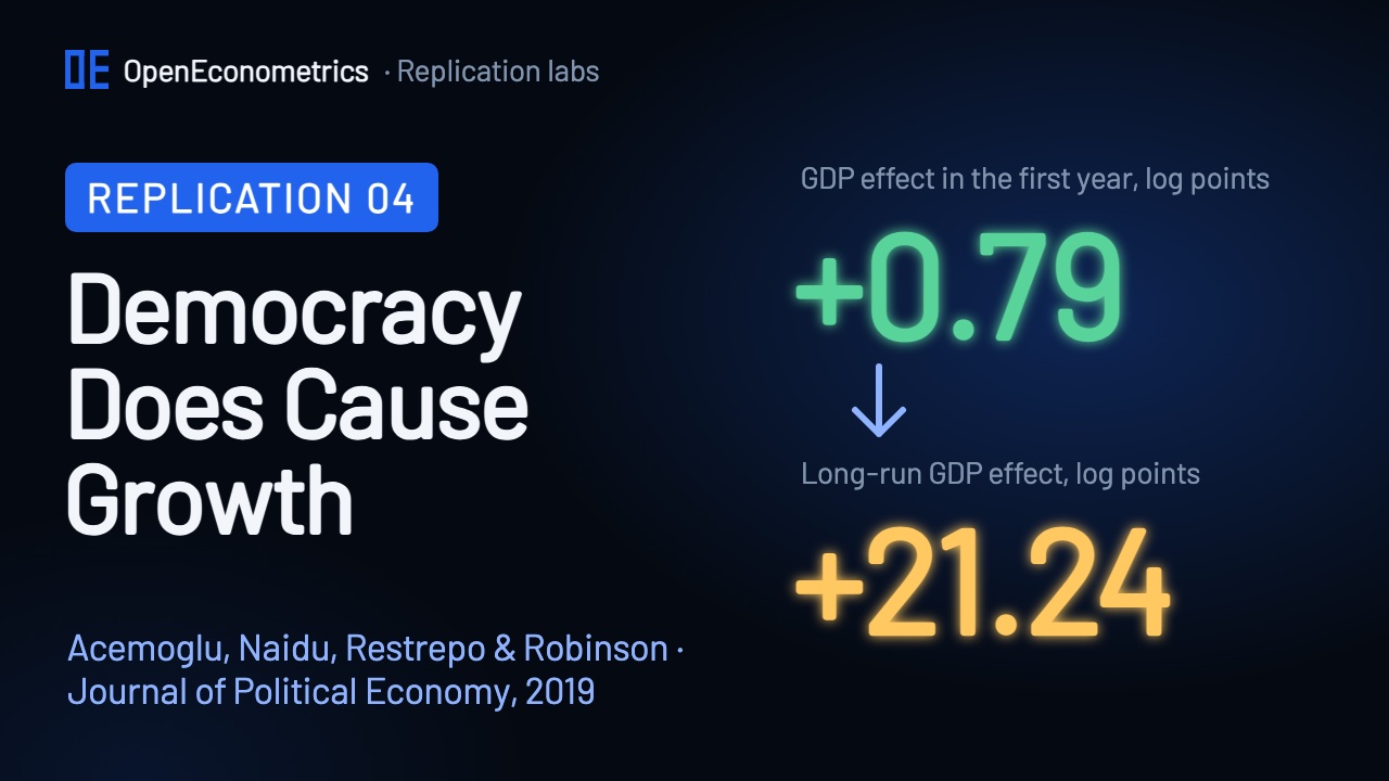
GDP is very persistent. In the preferred column the lag coefficients are 1.238, −0.207, −0.026 and −0.043, and they sum to 0.963. A permanent democratization adds β every year, and most of each gain carries forward, so the effect accumulates to the long-run effect β / (1 − Σγ): 0.787 / (1 − 0.963) = 0.787 / 0.037, which at full precision is 21.24 log points, 27 times the first-year effect.

The long-run effect is a nonlinear function of five coefficients, so its standard error comes from the delta method: the gradient of the function combined with the full covariance matrix of the estimates. In OpenEconometrics this is oe.nlcom(fit, lambda c: c["dem"] / (1 - c["L1_y"] - c["L2_y"] - c["L3_y"] - c["L4_y"])). The result, 7.21, is 32 times the standard error of β itself: dividing by a small number, one minus the persistence, magnifies every uncertainty.

The main result

Table 2, column 3 · within, 4 lags	Paper	This lab
Democracy	0.787 (0.226)	0.7866 (0.2263)
Log GDP, lag 1	1.238 (0.038)	1.2381 (0.0376)
Log GDP, lag 2	−0.207 (0.046)	−0.2065 (0.0458)
Log GDP, lag 3	−0.026 (0.028)	−0.0261 (0.0282)
Log GDP, lag 4	−0.043 (0.017)	−0.0425 (0.0173)
Long-run effect	21.240 (7.215)	21.2396 (7.2149)
Effect after 25 years	16.895 (5.297)	16.8953 (5.2968)
Persistence (sum of lags)	0.963 (0.005)	0.9630 (0.0052)
Observations	6,336	6,336
Countries	175	175

In the year of a democratization, GDP per person is 0.787 log points higher (standard error 0.226). The long-run effect is 21.24 log points (standard error 7.21; 95% interval 7.0 to 35.5), and after 25 years the effect is 16.9 (5.3). The sample has 6,336 country-years from 175 countries, with standard errors clustered by country as in Stata's xtreg, fe r. Every number in the column matches the paper and the authors' own output file at the printed precision.

The paper calls the long-run effect a "21.24 percent" increase. Because the outcome is 100 × log GDP, it is 21.24 log points; the exact percent change is exp(0.2124) − 1 = 23.7%. This page reports log points.

Long-run effectLower 95% boundUpper 95% boundEffect after h years (Figure 2)

The effect builds slowly: 0.79 log points in the first year, 4.9 after five years and 16.9 after 25, still rising toward the long-run effect. The 95% band stays above zero at every horizon. All 70 values the authors saved for this figure (30 effects with standard errors and the five coefficients) match the run to within 1e−9.

1 lag · persistence 0.97335.59 (14.00)

2 lags · persistence 0.96719.60 (8.60)

4 lags · persistence 0.96321.24 (7.21)

8 lags · persistence 0.96022.01 (7.74)

Within estimator, country and year fixed effects, standard errors clustered by country. Persistence is the sum of the lag coefficients.

With one lag, persistence is 0.973 and the long-run effect is 35.6 (14.0); with two lags, 19.6; with four, 21.2; with eight, 22.0. Lags 5 to 8 add nothing jointly (F = 0.74, p = 0.565), which is why four lags is the preferred model. In every column the long-run interval stays above zero.

Regional waves of democratization

Democracy spreads within regions: Latin America democratized in the 1980s and early 1990s, Eastern Europe and Central Asia after the fall of the Soviet Union. Table 6 instruments a country's democracy with the share of democracies among the other countries in its region (one of seven) that started the sample with the same regime, leaving the country itself out. The first four lags of this wave are the excluded instruments. The exclusion restriction is that, given its GDP history and the fixed effects, a regional wave affects a country's GDP only through its own democracy; a regional recession or trade collapse that moved both would break it, and the robustness columns control for such channels.

Regional wave, t−10.547 (0.101)

Regional wave, t−20.133 (0.081)

Regional wave, t−30.227 (0.067)

Regional wave, t−4−0.087 (0.110)

Dependent variable: democracy (0/1). Excluded-instruments F (Kleibergen–Paap) = 33.2.

The first lag carries most of the first stage: 0.547 (0.101). Ten more percentage points of democracy among a country's peers raise its chance of being a democracy the next year by about 5.5 points. The cluster-robust Kleibergen–Paap F statistic for the excluded instruments is 33.2, a strong instrument.

Two-stage least squares on 6,309 country-years from 174 countries gives a democracy coefficient of 1.149 (0.554) and a long-run effect of 31.52 (17.42). Both are larger than the within estimates but much less precise; the long-run interval reaches below zero. The Hansen test of the four instruments gives p = 0.21, no sign that they disagree.

(1) Wave t−1 only0.966 (0.558)

(2) Baseline (waves t−1 to t−4)1.149 (0.554)

(3) GDP in 1960 quintiles × year effects1.125 (0.689)

(4) Soviet dummies1.292 (0.651)

(5) Regional trends1.697 (0.885)

(6) Regional GDP and trade1.817 (0.663)

(7) Regional unrest, GDP and trade1.107 (0.656)

(8) Spatial lag of GDP1.335 (0.536)

(9) Spatial lags of GDP and democracy1.361 (0.895)

Democracy instrumented with lags of the regional wave; country and year fixed effects; standard errors clustered by country.

With only the first lag of the wave, the coefficient is 0.97. Adding GDP-quintile-by-year effects, Soviet dummies, regional trends, regional GDP and trade, regional unrest or spatial lags leaves it between 1.1 and 1.8. Five of the nine intervals include zero, but every estimate is positive. In column 9, with spatial lags of both GDP and democracy, the first stage is weak (F = 4.55).

Other estimators

With a lagged outcome and country fixed effects, the within estimator has a bias of order 1/T, the Nickell bias; here each country is observed 38.8 years on average. Table 2 therefore adds Arellano–Bond difference GMM (columns 5 to 8) and the HHK estimator of Hahn, Hausman and Kuersteiner (columns 9 to 12). This lab could not rerun either (see below), so the chart shows their printed values in grey.

Within · Table 2, col 321.24 (7.21)

Arellano–Bond · Table 2, col 716.45 (8.44)

HHK · Table 2, col 1125.03 (10.58)

2SLS · Table 6, col 231.52 (17.42)

Collapsed GMM · extension15.04 (19.11)

Blue: reproduced in this lab. Grey: the paper's printed values, not reproduced. Amber: an extension, not a paper target.

With four lags, Arellano–Bond gives 16.45 (8.44) and HHK 25.03 (10.58): every estimator points the same way. What the SDK can run is difference GMM with collapsed instruments, 145 of them on the paper's Arellano–Bond sample. As an extension, not a check of the paper, it gives a four-lag long-run effect of 15.0 (19.1): far fewer instruments, far less precision.

The scorecard

Target	Paper	This lab	Result
Table 2 · col 3 · democracy	0.787 (0.226)	0.7866 (0.2263)	✓ Match
Table 2 · col 3 · long-run effect	21.240 (7.215)	21.2396 (7.2149)	✓ Match
Table 2 · col 3 · persistence	0.963 (0.005)	0.9630 (0.0052)	✓ Match
Table 2 · col 4 · lags 5–8, p-value	0.565	0.5647	✓ Match
Table 6 · col 2 · 2SLS democracy	1.149 (0.554)	1.1494 (0.5541)	✓ Match
Table 6 · col 2 · long-run effect	31.521 (17.425)	31.5205 (17.4250)	✓ Match
Table 6 · col 2 · first stage, wave t−1	0.547 (0.101)	0.5470 (0.1008)	✓ Match
Table 6 · col 2 · excluded-instruments F	33.2	33.21	✓ Match
Text · SE after 25 years, col 1	5.7	5.6486	Rounding
Table 2 · col 4 · unit-root t statistic	−7.00	−6.9909	Difference
Tables 2 and 6 · cells rerun	244	243 match · 1 differs	Difference

Group	Numbers	Match	Rounding	Differ	Not reproduced
Table 2 · within (cols 1–4)	71	70	0	1	0
Table 2 · Arellano–Bond (cols 5–8)	67	0	0	0	67
Table 2 · HHK (cols 9–12)	63	0	0	0	63
Table 6 · A · 2SLS	107	107	0	0	0
Table 6 · B · first stages	66	66	0	0	0
Table 6 · C · HHK	90	0	0	0	90
Figure 2 · authors' saved estimates	70	70	0	0	0
Figure 1 · authors' plotted line	46	46	0	0	0
Numbers quoted in the text	34	27	3	0	4
Tables 2 and 6 · all printed cells	464	243	0	1	220

All 464 printed cells of Tables 2 and 6 were transcribed, and every one agrees with the authors' own .tex output files. Of the 244 cells that OpenEconometrics could rerun, 243 match at the printed precision. The other 220 belong to the Arellano–Bond and HHK estimators. Figure 2's 70 saved values and Figure 1's 46 plotted points match the authors' files. Of 34 numbers quoted in the text, 27 match, 3 differ only through the paper's own rounding and 4 belong to the estimators the lab cannot run.

• The one difference (unexplained). The unit-root t statistic of Table 2, column 4: the authors' own llctest program gives −6.991 on the archived data; the paper and the authors' file print −7.00. That row was typed by hand into the output file, and no rounding rule turns one into the other. The other three unit-root statistics (−4.79, −3.89, −4.13) and all four p-values match.
• Rounding in the text. The text quotes 5.7 for the printed 5.649 and 26.32 for 26.315 (rounding twice), and 17.07 for 17.075 (cut off rather than rounded).
• Units. Where the paper writes "percent", the numbers are log points; it also labels the standard error of the democracy coefficient "0.226 percent".

No coefficient, standard error, long-run effect or sample size of a reproduced column differs.

Where this replication stops

• Arellano–Bond, Table 2 columns 5 to 8. The SDK has the estimator (oe.xtdpd), but the paper's specification uses every available lag of GDP and democracy as an instrument, 2,550 instrument columns, and oe.xtdpd refuses specifications above 2,000. Every run of the lab checks and records that refusal.
• HHK, Table 2 columns 9 to 12 and Table 6 Panel C. The SDK has no HHK estimator. Together, these two estimators account for the 220 printed cells that are not reproduced.
• Tables 1, 3–5 and 7–8, Figures 3–6 and the online appendix are outside this lab.

The causal reading rests on assumptions a replication cannot test: sequential exogeneity for the within estimates and the exclusion restriction for the waves. Democracy is coded yes or no, so the indicator cannot see degrees of democracy and may be mismeasured.

Run it yourself

Watch the companion video above. The lab package will be published here. You will need the authors' files, which we never redistribute:

1. Run prepare_sources.py from the lab package. It downloads the authors' replication archive (10.3 MB) and the paper from Daron Acemoglu's data archive at MIT, extracts the 17 files the lab reads, and checks all 19 files against their recorded SHA-256 fingerprints.
2. Open a Python document in OpenEconometrics, point the launcher at the lab, the authors' files and a new results folder, and press Run.

from lab import run_lab

result = run_lab(
    source_root=source_dir,
    output_dir=results_dir,
    display_callback=display,
)

Each Table 2 column is one call, followed by oe.nlcom for the long-run effect:

fit = oe.xtreg(data=s, y="y", x=lags + ["dem"] + yy, panel="wbcode2", time="year", model="fe", covariance="robust")

The run writes reconciliation.csv, with every published number and every value from the authors' output files next to the lab's result.

The paper

Daron Acemoglu, Suresh Naidu, Pascual Restrepo and James A. Robinson, "Democracy Does Cause Growth", Journal of Political Economy 127(1), 47–100, 2019. doi:10.1086/700936. Data and Stata programs: Daron Acemoglu's data archive at MIT; no licence is stated for them. The paper, the authors' data and code keep their own rights; this page and the lab describe and recompute them.