Econometrics · Lab 17 of 20
The Trap of Trending Series
Stationarity, unit roots and spurious regression.
Two economic indices rise over several decades. A regression of one on the other gives an above 0.92 and an enormous t statistic. Is that strong evidence of an economic relationship, or can the shared appearance of upward movement produce a misleading result?
This lab examines two independent synthetic random walks with drift. Their innovations have no relationship and neither series causes the other. Nevertheless, their levels produce a striking regression. We then examine changes and use two native time-series tests whose null hypotheses point in opposite directions. The exercise connects the algebra of accumulated shocks to the practical question of what a regression's reported significance means.
All 240 quarters are supplied in trending_series.xlsx. No index is measured from an actual economy. The numerical results are real executions of OpenEconometrics on the simulated data, not an empirical claim about any pair of macroeconomic variables.
1. Start with what a shock does over time
Consider a stationary autoregression around a fixed mean:
A shock affects today's value and then decays. Its contribution periods later is proportional to . Under appropriate initialization and finite innovation variance, the series has a stable mean and variance, and its autocovariance depends on the lag rather than the calendar date. These are features of covariance stationarity.
A random walk behaves differently:
The coefficient on the lagged level is exactly one. Expanding the recursion shows why the distinction matters:
Every past innovation remains in the current level. A shock does not fade away. With independent innovations of variance , the random component has variance . Thus subtracting a deterministic linear trend does not make the accumulated stochastic component stationary.
This is the difference between a deterministic trend and a stochastic trend. A series can trend upward because its expected value follows a calendar pattern, because it accumulates permanent shocks, or because both mechanisms operate. A line on a plot cannot by itself distinguish those possibilities.
2. Understand the synthetic indices
The prepared indices were constructed from independent standard-normal innovations according to
The two innovation sequences are independent. Both indices have positive drift, but there is no behavioral equation linking them. The units are arbitrary index points; these are not percentages or currency amounts.
| Variable | Meaning | Sample |
|---|---|---|
quarter | Consecutive integer calendar index | 1–240 |
index_x | First independent random walk with drift | 240 levels |
index_y | Second independent random walk with drift | 240 levels |
change_x | Quarters 2–240 | |
change_y | Quarters 2–240 |
The first difference needs two observed levels, so it loses the first row. The resulting regression has 239 observations. The script retains the original quarter labels rather than silently pretending that the first change belongs to quarter 1. There are no missing interior periods, and all models use explicit missing="raise" where that argument is supported.
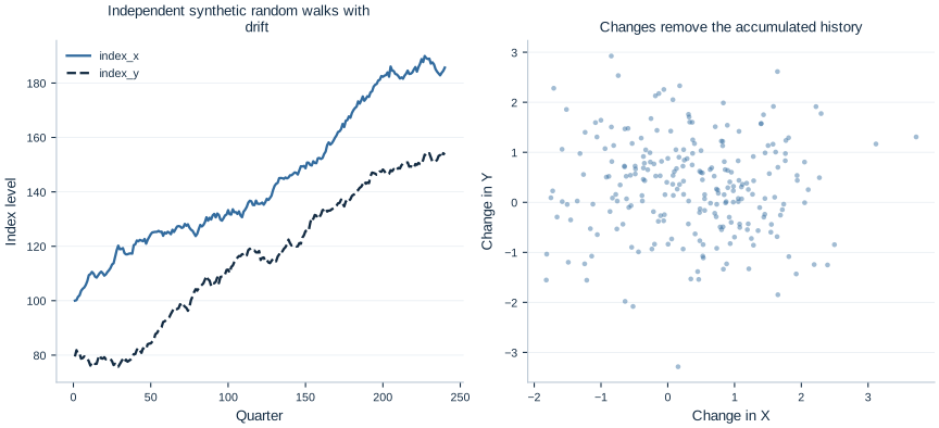
The levels panel shows long movements generated by drift and accumulated innovations. The changes panel asks a different question: when X has an unusually large increment in a quarter, does Y also have an unusually large increment? Independence of the innovations implies no population relationship between those increments, even though the levels appear to move together.
3. Fit the tempting level regression
Download trending_series.xlsx and lab.py. In OpenEconometrics, import the workbook without changing its filename, then open lab.py in a Python document and run the complete file. The workbook's first sheet, Data, contains the observations; Dictionary explains the variables and units.
The script reads the prepared indices, fits the level and change models, displays the native tests, and plots quarterly changes. Everyone using the supplied workbook starts from the same observations and obtains the same reported results.
In ordinary Python, keep the workbook beside lab.py and run python lab.py from an environment where OpenEconometrics is installed. To read a workbook from another folder, use from lab import run_lab, then call run_lab(data_path="/path/to/trending_series.xlsx"). The script writes no exports unless an output directory is explicitly supplied.
After the file has been run, inspect the level specification:
data = load_data()
levels = oe.ols(
    data=data,
    y="index_y",
    x=["index_x"],
    covariance="nonrobust",
    missing="raise",
    device="cpu",
)
print(levels.summary())
The executed regression reports
| Reported level-regression quantity | Value |
|---|---|
| Slope | 0.954429 |
| Conventional standard error | 0.017044 |
| Reported t statistic | 55.998 |
| Reported two-sided p-value | Approximately |
| 0.929455 |
The software has correctly calculated this least-squares line and its requested conventional formula. The problem is interpreting that formula under a data-generating process for which the usual stationary-regression reference argument does not apply. A tiny reported p-value cannot turn two independent accumulated processes into an economic mechanism.
High measures how much level variation the fitted line explains in this sample. It is not a test of causality, stationarity, or theoretical relevance. Likewise, adding significance stars to this table would decorate an invalid inferential interpretation rather than resolve it. The classic issue is discussed by Granger and Newbold.
4. Change the question from levels to increments
First differencing removes the accumulation:
The independent shocks remain independent. Create the change sample explicitly before fitting:
changes = data.assign(
    change_x=data.index_x.diff(),
    change_y=data.index_y.diff(),
).iloc[1:].copy().reset_index(drop=True)

model_changes = oe.ols(
    data=changes,
    y="change_y",
    x=["change_x"],
    covariance="HC3",
    missing="raise",
    device="cpu",
)
print(model_changes.summary())
The change slope is −0.015484, with HC3 standard error 0.067413, 95% interval [−0.148289, 0.117321], and p-value 0.8185. The change regression's is approximately 0.000268. These results are consistent with the independent increments that we deliberately generated.
The two slopes are not alternative estimates of an unchanged target. The level regression describes a relationship among accumulated index values; the difference regression describes the association between quarter-to-quarter increments. Its unit is “Y index-point change per X index-point change.” Differencing can be appropriate for an integrated process, but it can also discard economically important long-run information. Choosing a transformation must follow a model of the series and the research question.
5. Ask a unit-root question with ADF
The augmented Dickey–Fuller regression used for the level series is
The null hypothesis is a unit root, . The alternative has a negative coefficient on the lagged level, corresponding to mean reversion after accounting for the declared deterministic terms. The statistic is a t-like ratio for , but its null reference distribution is Dickey–Fuller, not the ordinary Student t distribution.
adf_level = oe.dfuller(
    data, "index_y", time="quarter", lags=1, trend="trend"
)
print(adf_level)
print(adf_level.attrs["critical_values"])
We include a constant and linear trend because the level process has drift and a trend-stationary alternative is relevant to the comparison. This choice changes the test specification and reference values; deterministic terms are not interchangeable formatting preferences.
For the level series, the statistic is −2.749939 and the approximate p-value is 0.21594. The 5% critical value is −3.429100. Rejection is in the more negative tail, so this result does not reject the unit-root null at 5%. Non-rejection does not prove a unit root; tests can have limited power against persistent alternatives.
For changes, the script uses one lagged change and a constant, without a linear trend. The statistic is −10.792592, with an approximate p-value of and a 5% critical value of −2.873814. This strongly rejects a unit root in the difference series under that specification. The level ADF regression uses 238 observations; the difference-series ADF regression uses 237, because constructing lags consumes additional rows.
The augmentation lag also has a purpose: it allows short-run dependence in changes to be represented before testing the lagged level. Too few lags can leave serially dependent auxiliary-regression errors; too many can consume observations and reduce power. This lab declares one lag as a transparent example rather than selecting it to produce a desired rejection. An actual analysis should explain lag selection and examine whether the resulting auxiliary regression has an adequate error specification.
Time ordering is equally substantive. The native test sorts by the declared quarter column and requires a consecutive calendar. An interior missing quarter cannot simply be dropped and treated as if its neighbors were adjacent: that would redefine the lagged variables. A time-series transformation must preserve the period it measures, just as a cross-sectional merge must preserve the observation it describes. Keeping sample counts alongside test statistics helps expose accidental changes in those definitions.
6. Reverse the null with KPSS
The KPSS test starts from stationarity as the null. With trend=True, the null permits a deterministic linear trend; with trend=False, it concerns stationarity around a level. A large statistic indicates that partial sums of detrended residuals are too persistent relative to the estimated long-run variance.
kpss_level = oe.kpss(data, "index_y", time="quarter", lags=4, trend=True)
kpss_change = oe.kpss(changes, "change_y", time="quarter", lags=4, trend=False)
print(kpss_level)
print(kpss_change)
The level statistic is 0.243405, above the trend-stationarity 1% critical value 0.216. The result rejects that stationary-trend null. The change statistic is 0.121466, below the level-stationarity 10% critical value 0.347, so it does not reject that null at conventional levels.
OpenEconometrics reports KPSS p-values using a bounded table interpolation. For these results, the notes state p < 0.01 for levels and p > 0.10 for changes. The stored boundary numbers 0.01 and 0.10 must not be described as exact tail probabilities. Reading the accompanying notes avoids overstating numerical precision.
Here ADF and KPSS tell a compatible story: persistent nonstationary levels and stationary increments. That agreement is useful evidence, not an automatic model-selection rule. Structural breaks, nonlinear dynamics, limited samples, and inappropriate deterministic terms can complicate both tests. When results conflict, examine the series and the specification rather than deciding that one test is always authoritative.
7. Understand what differencing does not solve
Replacing levels with changes does not create exogeneity, eliminate measurement error, or establish causal direction. Differencing a variable measured with noise may even make that noise relatively more important. It also changes interpretation from a level relationship to a short-run change relationship.
Some nonstationary series share a genuine long-run equilibrium: a particular linear combination can be stationary even when each individual series has a unit root. That possibility is cointegration. Independent random walks in this lab do not have a constructed common equilibrium. An empirical project with an economic long-run theory would need to investigate that theory rather than mechanically difference every variable and declare the problem solved.
Adding a time trend to a level regression can address a deterministic common trend but does not generally remove accumulated stochastic trends. Changing only the covariance estimator also does not repair the entire nonstationary regression problem. The model, transformations, sampling behavior, and reference distribution must fit together.
The level example is a substantive inferential failure even though its least-squares calculation is correct. Understanding that distinction is essential when a striking software output conflicts with the process that generated the observations.
8. Report a defensible comparison
The publication LaTeX table places the level and change models side by side, with their different outcomes and sample counts clearly labeled. That labeling matters because similar-looking columns can otherwise imply that a transformation merely changes precision around an unchanged target.
When communicating the lesson, report the level fit as a misleading example, the change estimate with its correct unit and sample, and the null hypotheses of the tests. Do not present non-rejection of a unit root as proof or claim that an insignificant change coefficient establishes that all economic connections are absent in every setting.
9. Questions for your analysis
- Expand a random-walk recursion and show why the variance of its accumulated innovation component grows with time. Contrast it with a stationary AR(1).
- Explain why the level regression's high and large t statistic are misleading in this constructed example. What does the software correctly calculate, and what interpretation fails?
- Derive the first differences of both generated indices. State the population slope expected in the change regression.
- Interpret the change coefficient and its confidence interval, including its units and the number of observations used.
- State the null and alternative of each test. Explain why ADF's statistic should not be compared with an ordinary t critical value.
- Explain the level and change KPSS results while respecting the bounds of the reported p-values.
- Describe a substantive situation in which differencing two nonstationary series could remove useful long-run information. What additional research question would need to be investigated?